Time and Tide: The Analysis of Degradation Data in JMP

[#1]

You’ve finally done it. After hours and hours (maybe days even), you’ve collected the measurements and are ready to analyze your reliability data in JMP. Someone mentioned this as being degradation data, so with a skip in your step, you hover over Analyze>>Reliability and Survival…and immediately stop in confusion. Repeated Measures Degradation? Destructive Degradation? What’s the difference? And what’s with the plain old Degradation platform? Which one do you use? What if you choose the wrong one and get misleading results? What if I lose my job and have to go back to working the dry docks with Bubba Gump and his shrimp boat?!!

Don’t worry. In this blog post, we’ll walk you through the highlights of each platform, showing you where each one is appropriate and where each has its limitations. Before long, you’ll be surfing through the analysis like a pro!

What is Degradation Data Anyways?

Let’s start with a core concept: degradation. If you’re reading this, you may already be familiar with it, in which case you can skip on to the next section. However, if you’re only familiar with life testing and/or need a refresher, then you’re in the right spot (though given it’s right after the intro, it wasn’t too hard to find…).

In typical life testing, you record the time you had to wait until the product failed or the patient recovered. With degradation testing, you actually measure some metric related to the product reliability or patient’s health that will change over time. This change is assumed to be monotonic; a fancy math term meaning that whatever direction it goes, it doesn’t change directions. So, for example, the capacitance of a capacitor will generally decrease or remain steady over time; it’ll never increase unless it is recharged. Alternatively, the degradation could be increasing, such as the amount of corrosion on a wire. In any of these cases, rather than waiting until complete failure, these metrics can be measured at certain time intervals until the end of the test. In fact, complete failure does not need to be observed at all! Instead, failure is typically defined as the value of the metric falling below or above a pre-defined threshold. This is called a soft failure.

Now that you (hopefully) get the concept of degradation data, let’s move on to the analysis.

To Destroy or Not to Destroy

There are two main categories of degradation data: repeated measures and destructive. An easy and fun way to remember the difference is to remember this question: “Have I seen you before?”. If you ask this of your subject and they respond “Yes”, then you are most likely dealing with repeated measures data. If they respond “No”, then you are most likely dealing with destructive data. If the subjects are actually inanimate objects and they still respond, DROP EVERYTHING AND RUN!!!!

In all seriousness, repeated measures data mean that each time you measure a subject, they go back into the study. With destructive data, a subject that is measured doesn’t go back. This is usually because the testing involves some damage or destruction to the subject (thus the name). But this doesn’t always have to be the case. The subject could be unharmed, but for some other reason cannot be returned to the study as the testing has changed something for them. A destructive degradation test typically requires more samples than a repeated measures test as you have to account for the sample pool decreasing over the course of the test.

Ultimately, the goal of any degradation analysis is the same as that for traditional failure analysis: to determine the distribution of failure times. With all degradation data, we use our understanding of how the data degrade over time to inform when they will fail, rather than relying solely on the times to failure. If a subject has not failed by the end of the test, we can use the estimated degradation path to predict when it would have failed, whereas in failure data, this subject would be censored. This makes degradation data more informative than failure data at the cost of a bit more work involved.

Degradation Data in JMP

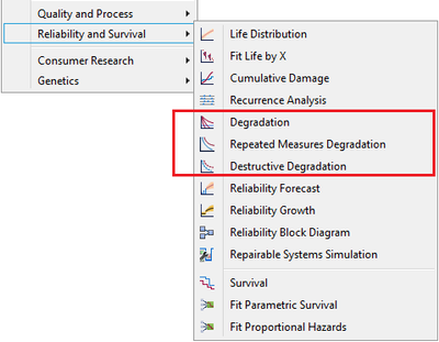
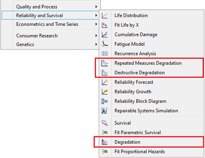
Ok, let’s get into the degradation analysis platforms in JMP. You can find all three platforms under the Analyze>>Reliability and Survival menu.

The following is a screenshot of the menu items in JMP 17.

The following is a screenshot of the menu items in JMP 18.

We’ll walk through each platform individually to highlight when it’s appropriate, how the analysis is conducted, and what are its limitations. We’ll then summarize our tour with some additional suggestions. If you’re looking for a more detailed look at each platform, we recommend you look into the Online Documentation.

Repeated Measures Degradation

What’s it for? As the name implies, this platform specializes in the analysis of repeated measures degradation data.

How does it work? You start by selecting from a wide array of degradation path models. This platform can also handle accelerated degradation tests, where the degradation path can change based on external factors. You can also include transformations of either the response measure or time or both. Next, you run a Bayesian estimation procedure to estimate the degradation path parameters, which can then be used to estimate a life distribution once you specify the soft failure threshold. You can fit multiple models to assess different fits. You can find more details in the documentation. 

What are its limitations? You must choose from the list of degradation path which, although pretty extensive, is not exactly comprehensive. You also must have some familiarity with Bayesian estimation (or at least be comfortable with the default settings) as there’s no option for alternative estimation methods.

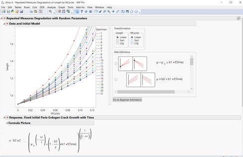
Example: To see an example of how the Repeated Measures Degradation platform works, check out the Alloy A data table in the Sample Data and run the table script. For an example that includes an acceleration factor, check out the Device B data table.

Destructive Degradation

What’s it for? As the name implies, this platform specializes in the analysis of destructive degradation data.

How does it work? You start by selecting from a wide array of degradation path models. This platform can also handle accelerated degradation models, in which case more path options appear that allow one or more of the parameters to be affected by the external factors. There are also transformations of either the response measure or time or both. Next, you run a maximum likelihood estimation of the path parameters, which includes diagnostic plots. Instead of specifying a single soft failure threshold, there are profilers that show the probability of reaching a specified response level. You can fit multiple models to assess different fits. You can find more details in the documentation. 

What are its limitations? You must choose from the list of degradation path which, although pretty extensive, is not exactly comprehensive. There’s also no option for alternative estimation methods beyond maximum likelihood.

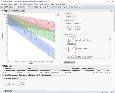
Example: To see an example of how the Destructive Degradation platform works, check out the Adhesive Bond data table in the Sample Data and run the table script.

Degradation

What’s it for? This platform handles both repeated measures and destructive data. It also has an option for stability tests, which are special tests used in pharmaceutical industries.

How does it work? You start by selecting transformations of the time and response axes. This platform assumes a simple linear path between (possibly transformed) inputs and outputs by default. If you have accelerating factors, you can also specify which of the degradation path parameters are affected. If the linear path is not appropriate, you have the option to specify a completely custom path model using a JMP Scripting Language (JSL) function called “Parameter”.

If you use the repeated measures part of the platform, the model is estimated using least squares. You can then specify thresholds to make inverse predictions, which produce soft failures. Those soft failures can then be analyzed using either Life Distribution, Fit Life by X (one acceleration factor), or Parametric Survival (multiple acceleration factors) to then determine the life distribution.

If you use the destructive degradation part of the platform, the model is estimated using maximum likelihood. You can then use the distribution profilers in the fitted model report to get the life distribution by controlling the failure threshold. You can find more details in the documentation.

What are its limitations? The repeated measures part of the platform follows the so-called pseudo-failure approach to analyze repeated measures degradation data. It requires two consecutive but separate analyses to get the lifetime distribution, whereas the standalone Repeated Measures Platform can produce the life distribution directly from a fitted degradation model. In addition, specifying your own model requires knowledge of JSL.

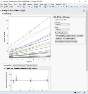
Example: To see an example of how the Degradation platform works, check out the Resistor data table in the Sample Data and run the table script.

Summary

Now that we’ve covered each platform, we hope your confusions have been cleared up and you’re more confident in your degradation analysis skills (no more dry dock for you!). Let’s summarize what we’ve learned:

• If you keep seeing the same subjects throughout the study, you’re working with repeated measures data. Your first stop should be the Repeated Measures Degradation platform. If it looks like the degradation path models there are too restrictive, then you can consider the Degradation platform instead.
• If the subjects have to leave the study after each test, you’re working with destructive data. Your first stop should be the Destructive Degradation platform. If it looks like the degradation path models there are too restrictive, then you can consider the Degradation platform instead.
• If you are conducting a stability analysis, then you should use the Degradation platform.
• If the degradation path that best describes your data is very specialized, you may want to consider the Degradation platform, since it can handle custom models.

Be sure to check out the JMP Online Documentation for details on how to use each platform as well as more examples. Should you still have questions, please reach out to our JMP Technical Support! And finally, don’t forget that analysis is best performed with a good helping of exploration and curiosity!