Multiple Linear Regression

[#1]

Use to model the relationship two or more continuous or categorical explanatory explanatory variables has with a continuous outcome variable. Useful to describe the relationships between the variables and to predict an outcome for different values of the explanatory variables.

Multiple Linear Regression Using Fit Model

1. From an open JMP^® data table, select Analyze > Fit Model.
2. Click on a continuous variable from Select Columns, and click Y (continuous variables have blue triangles).
3. Choose explanatory variables from Select Columns, and click Add. To add an interaction term, select the variables and click Cross. Here we included the sex*height interaction.
4. Click Run.

By default, JMP will provide the following output:

• Effect Summary
• Summary of Fit table.
• Analysis of Variance table.
• Lack of Fit table.
• Parameter Estimates table.

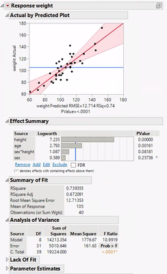
Note: default output can be changed via Preferences (File > Preferences) and selecting Platforms > Fit Model > Fit Least Squares).

• Select Estimates > Show Predicted Expression under the top red triangle to display an equation for the fitted model.
• To save the prediction formula, predicted values, residuals and other statistics to the data table, click on the top red triangle, select Save Columns.  JMP will create new columns in the data table.
• Model Diagnostic plots can be found under Row Diagnostics.
  Here we also added an Actual by Predicted Plot.
• To view indicator parameterization (using 0, 1 coding), select Estimates > Indicator Parameterization Estimates from the
  top red triangle.
• To view the effects of the explanatory variables on the predicted response, click on the top red triangle, select Factor Profiling and choose Profiler. In the Prediction Profiler, click and drag the vertical red line for a variable to change the level or value. The predicted mean response and 95% Confidence Interval are displayed.

Visit Discovering JMP > Analyze Your Data > Analyze Relationships and Fitting Linear Models in JMP Help to learn more.