Multiple Regression, Multicollinearity, and Model Building - Housing Prices

[#1]

Produced by: Marlene Smith

University of Colorado Denver Business School

Background

A real estate company that manages properties around a ski resort in the United States wishes to improve its methods for pricing homes.  Data is readily available on a number of measures, including size of the home and property, location, age of the house, and a strength-of-market indicator. 

The Task                 

After determining which factors relate to the selling prices of homes located in and around the ski resort, develop a model to predict housing prices. 

The Data        Housing Prices.jmp

The data set contains information about 45 residential properties sold during a recent 12-month period.  The variables in the data set are:

Price                             Selling price of the property ($1,000)

Beds                             Number of bedrooms in the house

Baths                            Number of bathrooms in the house

Square Feet                  Size of the house in square feet

Miles to Resort              Miles from the property to the downtown resort area

Miles to Base                Miles from the property to the base of the ski resort’s mountain

Acres                            Lot size in number of acres

Cars                             Number of cars that will fit into the garage

Years Old                     Age of the house, in years, at the time it was listed

DoM                             Number of days the house was on the market before it sold

 

Analysis       

This problem involves one response variable, the selling price of the home, and various potential predictors of selling price.  Three of the predictor variables measure, directly or indirectly, the size of the house: square feet, number of bedrooms and number of bathrooms.  Simple regression models were developed for each of these predictors.

Below are summaries for each of the models:

Model	RSquare	RMSE	P-Value
Price = 137.4 + 77.2 Beds	0.456	98.9	< 0.0001
Price = 141.8 + 106.9 Baths	0.640	80.5	< 0.0001
Price = 134.0 + 0.135 Square Feet	0.486	96.2	< 0.0001

The models indicate that, based on the single-predictor models, the house price increases by:

• $77,200 for each bedroom.
• $106,900 for each bathroom.
• $135 for each square foot.

Multiple regression (Exhibit 1) allows us to understand the simultaneous influence of the three predictor variables on the selling price.

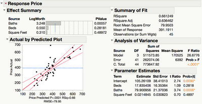
Exhibit 1    Multiple Regression for Price and the Three Size Variables

(Analyze > Fit Model; select Price as Y and the size variables as Model Effects, and hit Run. Some default output is not displayed, and the layout has been changed to fit better on the page.) 

Comparing the multiple regression model to the three simple regression models reveals that the coefficients have changed:

• $17,835 per bedroom in the multiple regression model, down from $77,200. 
• $79,900 per bathroom (formerly $106,900).
• $21/square foot in multiple regression, but $135/square foot in simple regression. 

In addition, the significance of each of the predictors has changed.  Two of the predictors that are statistically significant by themselves in simple regression models (Beds and Square Feet) are no longer significant when used in conjunction with other predictors.  The reason for this is the correlation among the predictors, or multicollinearity. 

As shown in Exhibit 2, the correlations among the predictor variables, which range from 0.728 to 0.7901, exceed the correlation between selling price and square feet (0.697) and between selling price and number of bedrooms (0.675). 

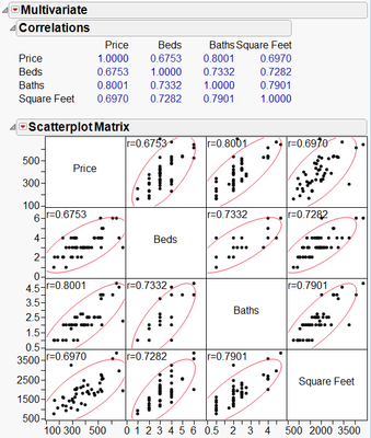
Exhibit 2    Correlations and Scatterplot Matrix for Price and the Size Variables

(Analyze > Multivariate Methods > Multivariate; select Price, and the size variable as Y, Columns, and hit OK.  Under the lower red triangle, select Show Correlations.)

In this setting, none of the correlations between the predictors are particularly surprising.  We expect square feet, number of bedrooms and number of bathrooms to be correlated, since adding a bedroom or bathroom to a house adds to its square feet.  The correlations are not perfect (i.e., equal to one) since adding square feet doesn’t always mean that you’ve added another bedroom or bathroom (you might have expanded the kitchen instead), and since adding a bedroom doesn’t always mean that you added another bathroom. 

Multicollinearity might also be anticipated between the two location measures: miles to the mountain base and miles to the downtown resort area.  Exhibit 3 suggests that there is indeed reason for concern, since there is high correlation between the two predictors (0.948).  This is evidenced in the scatterplot matrix by the density ellipses (Exhibit 3), which are much narrower than the ellipses involving the response, Price. 

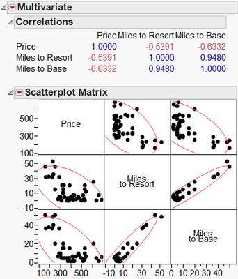
Exhibit 3    Pairwise Correlations and Scatterplot Matrix - Location Variables

In the simple regression models for the location variables, both predictors are highly significant and the coefficients are negative.

Model	RSquare	RMSE	P-Value
Price = 454.66 – 5.118 Miles to Resort	0.291	112.97	< 0.0001
Price = 473.61 – 5.925 Miles to Base	0.401	103.81	< 0.0001

The overall regression model involving the two location variables (Exhibit 4) is highly significant, with a p-value of < 0.0001 for the F Ratio.  Yet only Miles to Base is a significant predictor of Price (at the 0.05 level).  In addition, the coefficients have changed dramatically.  The coefficient for Miles to Resort is now positive! (Does selling price really increase as the distance to the resort increases?) Once again, we should be concerned with very high correlation between the two predictors, Miles to Resort and Miles to Base. 

Exhibit 4    Multiple Regression for Price and the Location Variables

We’ve found indications of multicollinearity with subsets of predictors, but let’s take a look at the multiple regression model using all of the predictors. 

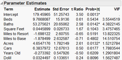
Exhibit 5    Multiple Regression for Price and All Predictors

(Right click over the Parameter Estimates table, and select Columns, VIF.)

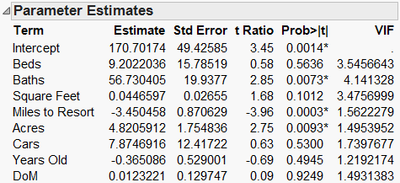
In the model above (Exhibit 5), only Baths and Acres are significant at the 0.05 level.  Are the other predictor variables not statistically significant due to multicollinearity?  A measure of the severity of the multicollinearity is the variance inflation factor, or VIF.  To calculate the VIF for a predictor (VIF_j), a regression model is fit using the predictor as the Y and the other predictors as the Xs.  The R² for this model (R_j²) is calculated, and then the VIF is calculated using this formula: 

An R_j² of 0.8 for a model predicting one variable from all of the other variables results in a VIF of 5, while an R_j² of 0.9 results in a VIF of 10.  So, a VIF greater than 5 or 10 is often considered an indication that the multicollinearity may be a problem.  (Note: This is not a firm rule of thumb – a Google search for VIF will yield many opinions on the subject).

The strong correlation between Miles to Resort and Miles to Base is clearly an issue.  In this situation, the multicollinearity might be alleviated by eliminating one of the two variables from the model.  In retrospect, it was discovered that the downtown resort area is close to the base of the mountain, meaning that these two variables are nearly identical measures of location.  Since Miles to Resort was deemed to be of greater practical importance than Miles to Base, only Miles to Resort will be used in the subsequent multiple regression model as a measure of location (Exhibit 6). 

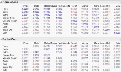
Exhibit 6    Multiple Regression for Price without Miles to Base

Three of the predictors (Baths, Miles to Resort and Acres) in the new model (Exhibit 6) are highly significant.  More importantly, the multicollinearity is now much less of a concern. 

Reducing the Model

Recall that the ultimate task, defined earlier, is to develop a pricing model.  The goal is to develop the simplest model that does the best job of predicting housing prices.  There are many ways to accomplish this; one approach is to simply remove non-significant predictors from the full model.  However, the significance of one predictor depends on other predictors that are in the model.  This makes it difficult to determine which predictors to remove from the model.  Tools like Stepwise Regression (covered in an exercise) provide an automated approach for identifying important variables and simplifying (reducing) the model. 

Here, we’ll reduce the model manually, one variable at a time, using p-values.  First, we revisit the correlations. 

The pairwise correlations (top report in Exhibit 7) show that some of the predictors are highly correlated with the response.  However, as we have seen, some predictors are also highly correlated with other predictors, making it difficult to determine which predictors are actually important.

Instead, we’ll use partial correlations.  A partial correlation is the correlation between two variables, while controlling for the correlation with other variables.  Partial correlations allow us to see correlations between each predictor and the response, after adjusting for the other predictors.  Notice how the correlations change (bottom report in Exhibit 7)!  For example, compare the pairwise and partial correlations for Beds and for Acres with Price.

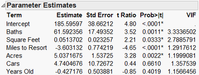
Exhibit 7    Pairwise and Partial Correlations

 (Analyze > Multivariate Methods > Multivariate; select Price and the remaining predictors as Y, Columns and hit OK.  Under the lower red triangle, select Partial Correlations.)

Four variables – Baths, Square Feet, Miles to Resort and Acres – have the highest partial correlations with the response.  Days on the market (DoM) and Beds have the lowest partial correlations. 

Since DoM also has the highest p-value (0.925 in Exhibit 6), we start our model reduction by removing DoM and refitting the model.  We then remove the variable with next highest p-value, Beds.

Note: When a variable is removed, the significance of the other variables may change.  So, non-significant variables should be removed only one at a time.

After removing these two variables, Cars and Years Old are still not significant, while Square Feet is now significant at the 0.05 level.  In addition, the p-values for the Baths, Miles to Resort and Acres have all decreased (Exhibit 8).

Exhibit 8    Parameter Estimates After Removing DoM and Beds

Continuing with this step-by-step approach, we eliminate Cars, then Years Old.  The final model is highly significant (the p-value for the F Ratio is < 0.0001), and remaining variables are all significant at the 0.05 level (Exhibit 9). 

Exhibit 9    The Reduced Model

Note: The approach taken here is essentially a manual form of backwards stepwise elimination, which is discussed in an exercise.

The final model (see the parameter estimates in Exhibit 9) estimates selling prices at:

• $53.64 per square foot.
• $65,560 per bathroom.
• $5,352 per acre.
• $3,644 less for each mile away from the resort.

Summary

Statistical Insights   

Multicollinearity and its impact on model building are the focus of this case.  Two predictors – distance of the house from the downtown resort area and distance to the mountain base – are nearly identical measures of location.  Eliminating one of these variables allows the other to remain statistically significant in a subsequent multiple regression model.

Examinations of pairwise correlations helped to uncover relationships that contributed to multicollinearity.  In more complex models, there may be intricate three- and higher-level correlations between the predictor variables that are difficult to assess.  The Variance Inflation Factor (VIF) is useful in signaling those cases. 

In practice, the final model developed in this case is highly significant, but could we do better? Are we missing other potentially important predictors?  For example, do we have a measure of the quality of the house and the building materials used?  And, how can we address the intangibles?  It is difficult to quantify subjective aspects of a house and neighborhood that might be key indicators of price. 

A Note About Model Diagnostics

When building a regression model, we need to verify that the model makes sense.  Three diagnostic tools commonly used are residual plots, Cook’s D, and Hats. 

• Residuals represent the variation left over after we fit the model.  Ideally, residuals (or studentized residuals) are randomly scattered around zero with no obvious pattern. 
• Cook’s D is a measure of the influence an individual point has on the model.  Observations with Cook’s D values >1 are generally considered to be influential.
• Hats is a measure of leverage, or how extreme an observation is with respect to its predictor values.  High leverage points have the potential to influence the model. 

We encourage you explore these model diagnostics on your own – we’ll revisit in an exercise.

Managerial Implications     

A statistical model tells us not to worry too much about garage capacity, age of the home and days on the market when it comes to estimating a house’s selling price in this particular market.  Being closer to the downtown resort area and mountain raises the selling price, and larger lots demand a higher price.

The statistical model developed for this analysis can be used as a crude way to identify which houses are statistically over- or undervalued.  Houses with large studentized residuals (greater than three) may be overpriced relative to the statistical model.  Likewise, houses with large negative studentized residuals (less than negative three) may be underpriced relative to the model – they might end up being great bargains!

JMP^® Features and Hints 

This case uses pairwise and partial correlations, scatterplot matrices and VIFs to assist in the identification of multicollinearity. 

VIFs are found by right-clicking over the Parameter Estimates table and selecting Columns, VIF. 

Since the significance of each predictor depends on the other predictors in the model, the model was slowly reduced using a combination of p-values and partial correlations.  Tools such as stepwise regression (a personality in the Fit Model platform) automate the model-building process.  Our one variable at a time approach is actually a manual form of backwards elimination, which is available in the stepwise platform. 

Exercises  

1.   Use the final model to predict the selling price for a 2,000 square foot home with two baths that is 15 miles to the resort and sits on one acre. 

Here are two ways to do this directly in JMP:

• In the Analysis window, select Save Columns > Prediction Formula from the top red triangle.  This will create a new column in the data table with the regression model.  Then, add a new row, and enter the values provided to predict the selling price.
• In the Analysis window, select Factor Profiling > Profiler from the top red triangle.  The Profiler displays the predicted response (and a confidence interval) for specified values of the predictors.  Click on the vertical red lines to change predictor values to those provided above.

2.    This case uses a manual backward model reduction approach, in which the full model (i.e., the one using all of the predictor variables) is reduced one predictor at a time based on statistical significance.  Let’s consider a different approach – forward model selection. 

Begin with a one-predictor model, perhaps based on the predictor with the highest correlation with Price or the lowest simple regression p-value, and add new predictors one at a time.  As you add predictors, examine the results under Summary of Fit, Analysis of Variance and the Parameter Estimates table. 

Do you arrive at a different final model?  If so, which model is preferred?   

3.    Open the data table FuelEfficiency2011.jmp (available for download from the Business Case Library at jmp.com/cases).  This data table contains information on a random sample of 2011 car makes and models sold in the US.

We’ll start by getting familiar the data.  Then, we’ll fit a model for MPG Highway and explore model diagnostics: residuals, Cook’s D influence, Hats, and multicollinearity.  Finally, we’ll use the JMP Stepwise procedure to explore different methods for building and selecting regression models. 

Part 1: Get to know the data

1. Use the Distribution platform to explore all of the variables (except Make and Model).  Describe the shapes of the distributions.
2. Use Analyze > Multivariate Methods > Multivariate to explore the relationships between the continuous variables.  Are any of the variables correlated with the response, MPG Highway? Are any of the variables correlated with other variables?

Part 2: Build a model, and explore model diagnostics

1. Build a multiple regression model using Fit Model, with MPG Highway as the response and all of the predictors as model effects (don’t include Make and Model), and run this model.
2. Explore the residuals.  (These are displayed by default.  Additional residual plots are available from the red triangle, Row Diagnostics). 

Are there any patterns or unusual observations?  Describe what you observe.

• Check Cook’s D Influence and Hat values.  (Select these options from the red triangle under Save Columns.  New columns in the data table will be created – use the Distribution platform to explore these values). 

Do there appear to be any influential or high leverage points?

• Check VIFs.  Does there appear to be an issue with multicollinearity? Use the Multivariate > Multivariate platform to explore bivariate correlations.  Do any of the variables appear highly correlated with one another?  

Part 3: Reduce the model using Stepwise

Return to the Model Specification Window.  Change the personality to Stepwise and click Run.  In this exercise, we’ll explore the different stopping rules and directions.

Note that this model includes one nominal variable, Hybrid?, which has strange labeling in the Current Estimates table.  JMP codes nominal variables as indicator columns – the labeling lets us know that coding has been applied.

• The default Stopping Rule is Minimum BIC.  Click Go.

The predictors selected for the model are checked as they are entered under Current Estimates.  Which terms have been selected for the model? 

• Click Remove All, change the Stopping Rule to Minimum AIC, then click Go. 

Which terms have been selected for this model?  Compare this model to the model found using Minimum BIC.

Note: BIC will tend to select models with fewer predictors, while AIC will tend to result in models with more predictors.

• Now, change the Stopping Rule from Minimum AIC to P-value Threshold.

The default selection routine, under Direction, is Forward.  Click Go. 

• Change the direction from Forward to Backward.  Click Remove All to deselect predictors and then click Go. 

Which terms have been selected for this model? Are the results different from Forward selection? Are different predictor variables chosen depending on the method used?

Note: Once predictors have been selected in Stepwise, select Make Model or Run Model to create the regression model.