Developer Tutorial: State-of-the Art Use of Repeated Measures Degradation to Model Product or Part Failures

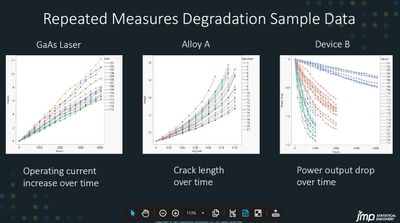
Repeated degradation data measures the reliability over time of a product such as propagation of cracks in a material, decrease in output of power amplifiers or other performance measurement changes over time on individual subjects. The goal of degradation modeling and analysis is to predict the failure times and probabilities for the product under study.

Beginning with JMP 17, JMP offers two different approaches for repeated measures degradation data analysis and modeling: 1) pseudo-failure approach that has been available in JMP Degradation platform for several releases and 2) a new Repeated Measures Degradation platform that implements the hierarchical Bayesian modeling for reliability discussed in Meeker, Escobar and Pascual (2022).

The hierarchical Bayesian modeling approach enables you to estimate degradation models with random parameters with Bayesian inference and find failure times through Monte Carlo simulation. It fits degradation path models with random parameters, whereas the pseudo-failure approach approach fits fixed parameter models. The hierarchical Bayesian modeling simulates the failure times using the posterior estimates of population parameters of the degradation path model, whereas the pseudo-failure approach extrapolates the pseudo failure times from the fixed parameter path model.  

In general, use the new Repeated Measures Degradation when one of its supported models is appropriate. If you don't see any models in the new platform appropriate for your data, you should consider using the pseudo-failure approach in the existing Degradation platform, where you can define your own model.

See a video that gives three case studies using JMP Sample data (GaAs Laser.jmp, Alloy A.jmp and Device B.jmp respectively) found in the Reliability folder of your JMP Sample Data. 

Question and answers are included after each case study. Case Study 1 begins at ~Time 24:00 , Cast Study 2 begins at ~ Time 57:00 and Case Study 3 begins at ~ Time 1:04:00.

Questions answered by Peng  Liu @peng_liu , Caleb King @calking  and Don McCormack @DonMcCormack at the live webinar:

Q: On the slide Repeated Measures Degradation Sample Data, in the 3 examples all the curves start at the same point. Is this a requirement for this type of study?

A: No, the curves need not start at the same point. A similar model but allowing random starts is next to the one with fixed start in the Path Definition list.

Q: Although these are all examples from manufacturing,  could this be used for an experiment in which you are stress-challenging animals over time (in which their health is “degrading” towards a “failure” = death)? I know there are survival-related analyses in JMP Pro, though this seems different.

A: Yes. Usually when you’re dealing with living entities,  we call it survival analysis. Similar techniques can be used. The main thing to consider whether this type of analysis is applicable is that (1) there are multiple subjects (2) repeated measurements are taken from individual subjects over time. There may not may not be a stress factor. But if there is one, this stress factor is expected to be constant on individual subjects over the entire time. The factor level can be different from subject to subject.

Q: Is there a way to handle two or more degradation response metrics (eg., current and voltage).

A: Currently, there is no way to do this in Repeated Measures Degradation. The trick would be how to combine the responses and their relationship to one another. Competing causes can be used to model the data given hard failures, but I am not sure about soft failures. And there are other techniques that can be used if the failures are from different failure distributions (e.g., defective subpopulations). There may still be a way to use competing causes with soft failures. You'd still estimate the failure distribution under each cause much like you would with hard failures. The difference is in how you get those estimated distributions. Once you have them though, I imagine the procedure would be the same.  Currently, there is no way to do this in Repeated Measures Degradation. See video ~time 1:16:00.

Q: If the Seed is Random, why do we all have the same random seed of 32323?

A: The label Random Seed is meant to imply "seed for random generation", not necessarily that the seed is itself random.

Q: Very specific question: Is there a way to use a degradation function like this: Performance parameter = a x exp (-(time/b)^c), i.e., with three parameters a, b and c and parameter a possibly being set the same for all devices?

A: This can be done using Degradation > Repeated Measures Degradation (i.e., the older platform).

Q: Can you use data filters in this platform?

A: Given that it is an iterative model, the model will not update if data filter is used. Data Filter is a general feature. It is kept available in the platform. The implication of using it, however, should be carefully considered. The current implementation leaves the decision to users. To be noticed, this is a time-consuming methodology, a change to the filter will trigger a non-trivial re-run of the analysis.

Q: Is there a way to use an acceleration model with two stress variable, e.g., temperature and current?

A: Not in new Repeated Measures Degradation platform, but you can add two stressors using the older Repeated Measures capability in Degradation platform. For hard failures, you can also use Fit Parametric Survival.

Resources

• William Q. Meeker, Luis A. Escobar, Francis G. Pascual, Statistical Methods for Reliability Data (2^nd edition), Wiley, 2022

• JMP documentation on Repeated Measures Degradation