Modify a Report Based on Analysis Results

[#1]

This recipe is motivated by material in the Display Trees chapter of the Scripting Guide. We will fit several models using the Bivarate platform and modify the report based on the results. The recipe shows how to navigate a report window to find the elements of interest. The Properties Window is used to show how to identify the object class name of report elements. A basic overview of working with colors in graph elements is also given.

---

Ingredients:

• Platform Objects
• Report Objects
• Scripting Index
• Colors
• XPath

Sample Data Tables – Big Class

Difficulty – Medium

Video Length – 4:56

Steps:

1. Open a new script window. Start with Names Default to Here(1); at the top.
2. Open the Big Class from the sample data directory. Copy the code from the enhanced log assigning a table reference to it.

   dt = Open( "$SAMPLE_DATA/Big Class.jmp" );

3. Launch the Fit Y by X platform with weight as Y and height as X. Select Fit Mean, Fit Line, and Fit Polynomial > 2, Quadratic from the hotspot. Directly below the graph, to the left of Linear Fit, use the hotspot to change the line color to the middle blue choice, 4^th from the bottom and Line Style to the third option. Change the color of the polynomial fit line to the middle orange option and the second line style.
4. Close the Bivariate Fit report. The code for the report window with all the changes appears in the Enhanced Log. From the hotspot at the top left, select Save Script > To Script Window.
5. Open returns a reference to the opened data table. Add a variable reference.

   tblRef = Open( "$SAMPLE_DATA/Big Class.jmp" );

6. Replace the hard coded table reference with the variable reference created above. The Bivariate platform message returns a reference to the platform. Create a variable to capture it.

   bivariatePlt = tblRef << Bivariate(…

7. Add Ignore Platform Preference(1) as the first argument to Bivariate. This will override any user selected platform preferences.
8. Add the following three lines below Bivariate. The messages are identical to their associated arguments in Bivariate and will be used to replace them. Delete the arguments from the Bivariate message otherwise the fits will appear twice each.

   biv << Fit Mean({Line Color( {212, 73, 88} )});
   biv << Fit Line({Line Color( "Blue" ), Line Style( "Dashed" )} );
   biv << Fit Polynomial(2,{Line Color( "Orange" ), Line Style( "Dotted" )});
   

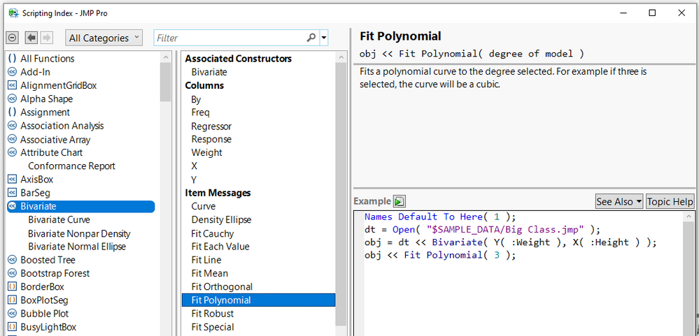
   Using messages instead of arguments to control report output gives us a simple and compact way to implement options. We could, for example, check for certain conditions using an If statement and decide whether the option should be turned on based on the results. In most cases, arguments and messages will be identical as seen above. To double check, we can look up the Bivariate platform object in the Scripting Index.

   

   Color and line style keywords can be specified with or without quotes and are not case sensitive. The Solid line style is default and does not need to be added.

9. Replace the list of three numbers in the Fit Mean message with the word “Red”. Quotes are optional and case is ignored.

   bivariatePlt << Fit Mean( {Line Color( Red )} );

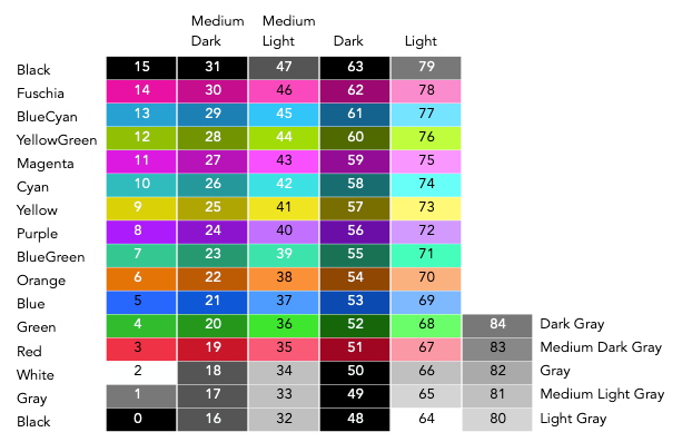
   We can specify line colors using one of 67 names, a three number list corresponding to red, green, and blue values, or a single value between 0 and 84. Names and numbers are given in the graph below.

   

   Colors in the 2^nd though 5^th columns are prefixed with the name at the top of the column. For example, 73 is Light Yellow, 9 is Yellow and 25 is Medium Dark Yellow. The short column at the far right contains shades of gray, the names of which appear at their right. Of the 85 color numbers, 67 are unique. The grays and Black are duplicated. 65 of the 67 colors appear in the color pop-up palette.

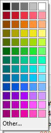
   The JMP color palette

   The order of the colors from top to bottom are, starting in the second row, Red, Orange, Yellow, YellowGreen, Green, BlueGreen, Cyan, BlueCyan, Blue, Purple, Magenta, and Fuchsia. The shades go Dark, Medium Dark, (no prefix), Medium Light, and Light. The five grayscale colors in the top row are Black, Dark Gray, Gray, Light Gray, and White. Medium Dark Gray and Medium Light Gray do not appear in the palette. For even more choices, you can specify a three-value list giving the red, green, and blue values of the color. Values can be specified on a either a 0 to 255 or 0 to 1 scale. For example, periwinkle is {204,204,255} (according to Wikipedia).

   The names for the Line Styles are Solid, Dotted, Dashed, DashDot, and DashDotDot.

10. Create a reference to the report layer of the analysis.

    bivariateRpt = bivariatePlt << Report;

    Alternatively, the Report function could have been used.

    bivariateRpt = Report(bivariatePlt);

    In general, visual report components are part of the report layer whereas analytical components are part of the platform.

11. We will use XPath to create a reference to every Parameter Estimates outline box to check the p-values.

    paramEstOutBoxes = bivariateRpt << XPath("//OutlineBox[text() = 'Parameter Estimates']");
    

    Since we have more than one Parameter Estimates outline, we want an easy and reliable way to reference all of them. Xpath is an open-source expression language developed by the World Wide Web Consortium standards organization.

12. We will loop through each of the Parameter Estimates outlines and check the last value in the last column of the table. If it is below a prespecified value, we will remove the fit. Let’s specify the value as a variable at the top of the script just below Names Default to Here.

    alpha = 0.05;

13. Loop using For Each

    For Each({paramEst,i},parEstOutBoxRefs,
    	nextPValues = paramEst[Number Col Box(4)] << Get;
    	If(nextPValues[N Items(nextPValues)]>alpha,
    		/*Code to Remove Fit*/
    	);
    );
    

    Get returns the entire column as a list.

14. If we were doing this interactively, we would go to the hotspot associate with the fit and select Remove Fit. Let’s start by assuming it is part of the platform. If we tried to send the Remove Fit message directly to the platform reference, nothing would happen. We can use the Scripting Index to get more information.
    1. Type remove fit in the search box at the top. In the list box directly below all items with either remove or remove fit appear.
    2. Select the first Remove Fit and scroll through the list using the down arrow. In the list box on the left, the objects associated with the entry are highlighted. The seventh Remove Fit entry is associated with Bivariate.
    

    The syntax at the upper right shows us how to use it.

    bivariatePlt << (Curve[i+1] << Remove Fit);

    We need to use i+1 to reference the curve because Fit Mean does not have a Parameter Estimates box. This should give use the code we need.

Hints for Success:

• Colors can be implemented as a name or in a list of red, green blue values.
• XPath is a flexible tool for finding object in a display tree.
• When in doubt about messaging, search the Scripting Index.