Using JMP to Find the Area Under a Curve

sseligman · Jun 19, 2023 10:00 AM

A common question users ask is how to use JMP to find the area under a curve. In this blog post, I’ll review a few possible ways to do so in JMP.

If you have X and Y coordinates of data, you can use the trapezoidal rule method. Below, I’ll work through an example of finding the area under a plasma concentration time curve. The data contains values of time (Time) and the associated concentration (C) of a drug in a subject’s blood at each time point. The content in this example comes from Nicole Jones’ piece in the Fall 1997 issue of JMPer Cable (see attached PDF copy).

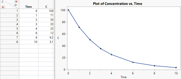
Figure A illustrates the data and the plasma concentration time curve.

The reference for this data is:

Bourne, D.W.A. (1995), “A First Course in Pharmacokinetics & Biopharmaceutics”, University of Oklahoma College of Pharmacy. http://157.142.72.143/gaps/pkbio/Ch04/Ch0403.html

Figure A. Data and Plot of Concentration vs. Time

In this example, we use a variation of the Trapezoidal Rule. The first step is to divide the time curve into segments between each time point. Then, we’ll calculate the area in each segment. Finally, we’ll add the pieces together to obtain the total area under the curve.

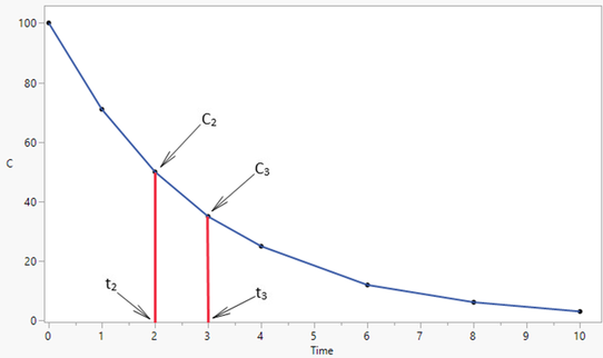
Consider each time segment to be a trapezoid, with its area given by the segment’s width and the average concentration within the segment width. Define t_i as the i^th time point (the unit of time is hours) and C_i as the drug concentration at the i^th time point. The concentration between the second and third time period, denoted as AUC_2,3and illustrated in Figure B, is computed as:

Figure B. Concentration vs. Time in Segments

This process works for all segments except the last - the time segment from 10 hours (in this example) until the drug has completely dissolved. The area under the last segment C_n can be calculated using the elimination rate constant (kel), computed from the sample data.

The kel constant is the negative slope of the relationship of the log of concentration and time. It is computed in JMP using the standard formula for the slope in a simple linear regression of Y on X:

For this example, the steps are as follows:

1) Create a new column in the data table (let’s call it ln(C)) and use the Natural Log function in the calculator (under Transcendental functions) to compute the log of the concentration.

2) Create another new column (let’s call it beta) and use the calculator to compute the slope parameter of the regression of time on ln(C), as shown below.

The calculator formula to compute beta uses an assignment function to create temporary variables for the numerator (XY) and for the denominator (x2) of the slope computation. It then computes and assigns XY/x2 as beta.

The last step is to compute the total area under the curve by summing the areas of the individual segments and that of the final segment, computed as:

If you’d like to reuse the data table containing these formulas as a template, simply delete all the rows and save the empty table with its formulas preserved. To use the template, simply open it and paste your data into the columns Time and C. Rename the columns to suit your data if needed, and the preserved formulas will automatically use the new column names and compute the total AUC.

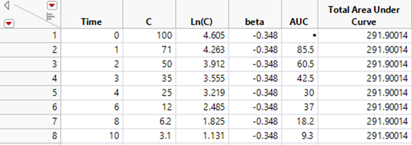
Figure C. Computed Slope Parameter and Total AUC

The data table shown in Figure C is attached to this post as well. It contains the necessary intermediate columns along with the total AUC calculation, and it includes all underlying formulas.

Another common question we receive is how to find the AUC when fitting a smooth curve to the data. You can use JMP to fit a smooth curve, and then use the trapezoidal rule to estimate the total AUC. Both the Fit Y by X platform and the Graph Builder platform can apply these fits.

The steps using the Graph Builder platform are as follows:

Create a scatterplot of your data in Graph Builder (see documentation here if you need help getting started).
Right-click within the graph and choose Add > Smoother. A smoothing function appears on the graph, along with a “Smoother” control panel to the left of the graph. By default, the method is set to Spline. You can use the slider to adjust the lambda value or right-click on it to set a specific value.
With your settings as desired, right-click in the graph and choose Smoother > Save Formula. The Spline prediction formula is saved to the original data table.
From the data table, go to Graph > Profiler and specify the new formula column in the Y, Prediction Formula role and click OK.
From the Prediction Profiler red triangle menu, set the Default N Levels option to a large number, like 10,000.
Then, from the red triangle menu, select Output Grid Table, creating a table of coordinates along the curve.
Using the coordinates produced in the grid table, we can use the trapezoidal rule to approximate the total area under the curve.

An example table called AUC_GridTable.jmp is attached. It was produced via the method above and contains 10,000 rows. There are two columns that each contain a total AUC value. The first is named Total AUC – Wikipedia Formula and uses the trapezoidal rule formula from Wikipedia (see this page). The second is called Total AUC – JMPer Cable and uses the formula from the first method discussed in this blog post. The intermediate columns needed for that method are also present. The two total AUC columns give similar approximations.

Lastly, if you want to find the area under the curve for a specific function, you can use numerical integration using Simpson’s Rule. A custom JSL script that performs the integration is attached (Integrate_Simpson Rule.jsl). Simply provide the function you want to integrate along with the upper and lower limits of integration.