- JMP User Community
- :
- Blogs
- :
- JMPer Cable
- :
- Genetic Association with JMP Genomics, Part 2: Basic Genetics Workflow (Case-Con...
- Subscribe to RSS Feed
- Mark as New
- Mark as Read
- Bookmark
- Subscribe
- Printer Friendly Page
- Report Inappropriate Content
JMP Genomics has analytical pipelines or Workflows to perform a series of analyses on a data set. The Basic Genetics Workflow is a quick and easy method for gaining a deeper understanding of your data before beginning a more in-depth analysis. This workflow recodes marker data to a numeric format, imputes missing genotypic data, and creates data subsets based on minor allele frequency (MAF), missing genotype proportions, and Hardy-Weinberg Equilibrium (HWE). The workflow then gives Marker Properties output and performs a Case-Control Association to identify markers of interest. Note that in this workflow, the case-control analysis is only useful for a binary phenotypic variable (affected vs. unaffected). For continuous or discrete phenotypic variables, other analyses such as the SNP-Trait Association (which will be covered in a later post) are more appropriate. In this example, we explore ~22,000 markers in a sample of 474 Bernese Mountain Dogs that are either affected or unaffected for histiocytic sarcomas (tumors).
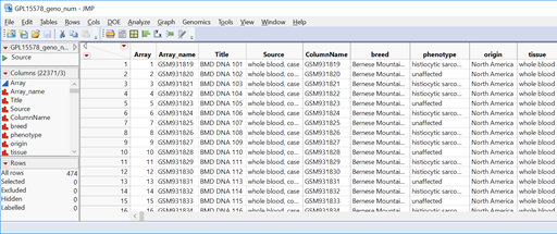
- Open the data set sas7bdat and inspect it. Note that the phenotype column has two levels: “histiocytic sarcoma” for dogs with a tumor and “unaffected” for dogs without. These need to be recoded as a binary (0 or 1) variable.
- For more information on how this data was imported to JMP, see the previous post in this series: Genetic Association with JMP Genomics, Part 1: Importing and Cleaning Data.
- For more information on how this data was imported to JMP, see the previous post in this series: Genetic Association with JMP Genomics, Part 1: Importing and Cleaning Data.
- Highlight the phenotype column by clicking on the column header cell. On the toolbar above the data, click the Recode icon (highlighted below). This tool allows for a quick recode of all levels in a given column.
- When the resulting window opens, enter 0 for unaffected phenotypes and 1 for HS phenotypes in the New Values column, then click Done. A drop-down menu will appear with options for including the new column in the data set. Select In Place to replace the old phenotype column with the newly recoded one. Save the data set, as it will be used as input for the workflow.
- With the binary phenotypic data now saved, return to the Genomics Starter menu and select Workflows > Basic > Basic Genetics Workflow.
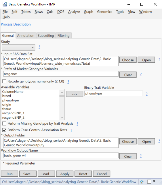
- In the General tab, select the newly saved sas7bdat as the Input SAS Data Set.
- In the box labeled Prefix of Marker Genotype Variables, type in “recgeno:” to specify that all column names starting with that string of characters contain marker data.
- As part of this workflow, non-numeric genotypes can be recoded by checking the Recode genotypes numerically.This data set already has numerically coded genotypes.
- Next, select the phenotype column as the Binary Trait Variable.
- The check boxes below the Available Variables box specify types of analyses to be run. For this example, select only Perform Case-Control Association Tests.
- Select an Output Folder and specify basic_gene_wf as the Workflow Output Name.
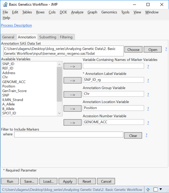
- On the Annotation tab, select the file sas7bdat as the Annotation SAS Data Set.
- Select the column SNP_ID_rg as the Annotation Label Variable, Chr as the Annotation Group Variable, and Position as the Annotation Location Variable.
- Optionally, select GENOME_ACC as the Accession Number Variable.
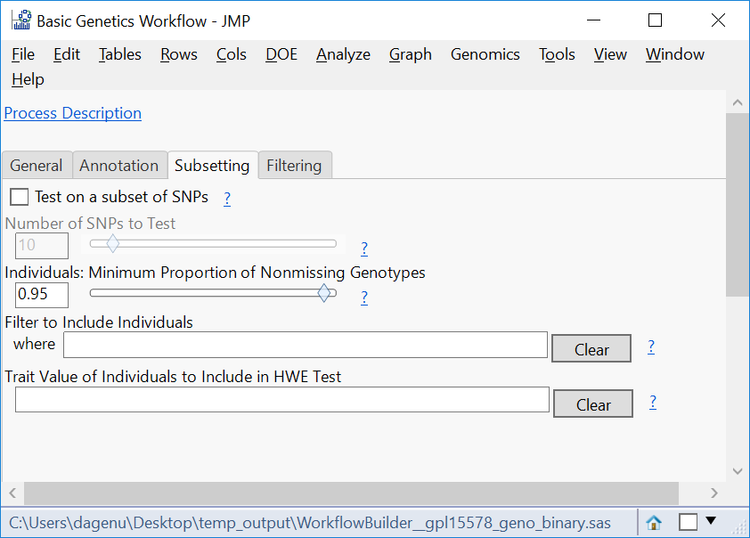
- The Subsetting tab gives options to filter individual samples (rows) from the data set. This can be done by testing a subset of SNPs or on every SNP and is filtered by a Minimum Proportion of Nonmissing Genotypes. In this case, enter 95 in the box to only include individuals with 90% or greater of their data present in the table.
- Note that exceptions to this filtering can be made in the Filter to Include Individuals where
- Leave the Trait Value of Individuals to Include in HWE Test blank to include the entire population in the test. The phenotypic value for affected or unaffected individuals can be entered here to only perform the HWE test on individuals of that phenotype.
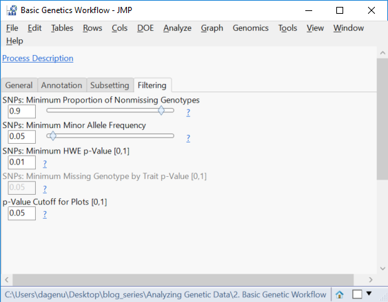
- Open the Filtering This tab gives options to remove SNP data (columns) with a low MAF, too many missing genotypes, or one that is likely not in HWE. Set the Minimum Proportion of Nonmissing Genotypes to 0.9, the Minimum Minor Allele Frequency to 0.05, and the Minimum HWE p-value to 0.05.
- Set the p-Value Cutoff for Plots to 05. This sets the threshold for determining which markers are significant.
- Click Run to begin the analysis.
Results
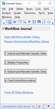
- The output window will be a JMP Journal (shown below) with each of the four analyses from the workflow. Each of the results is clickable and opens a new window with the results from that analysis. Note that this journal can be reopened and the results reexamined at any time as long as the files aren’t moved from their specified Output Folder.
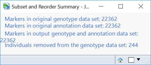
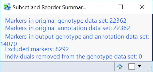
- Click the first result Subset and Reorder Genetic Data. The window below will appear giving a summary of the number of markers and individuals in the subset. The criteria for this subset was specified in the Subsetting tab and has removed 244 individuals with less than 95% of nonmissing data.
- Click the Open buttons next to each data set to open them. The top set is the genotypic subset, and the bottom set is the corresponding annotation subset.
- Return to the journal and open the Marker Properties results.
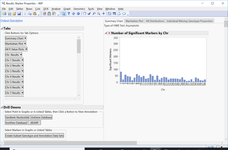
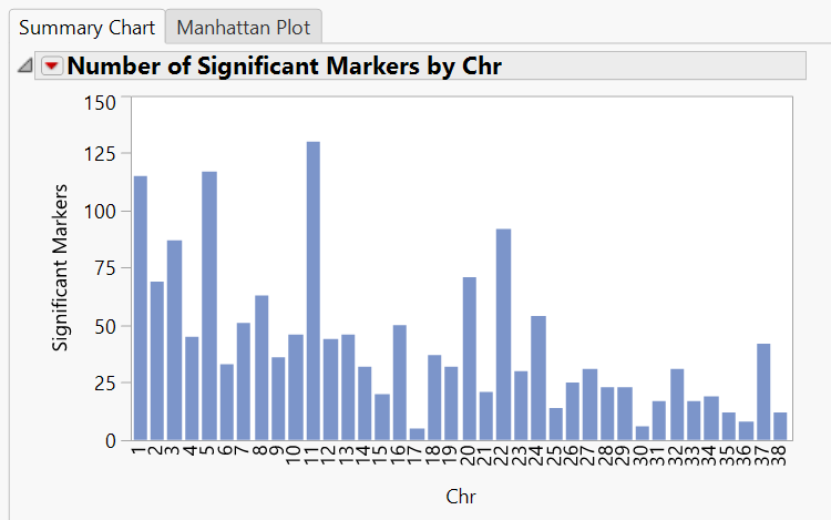
- The initial tab gives a Summary Chart of significant markers by chromosome for Hardy Weinberg Equilibrium.
- Note: Each of the bars on the graph can be selected and subset in the Drill Downs Simply select the bar corresponding to the desired chromosome, highlight it, and click Create Subset Genotype and Annotation Data Sets on the left of the window under the Drill Downs heading.
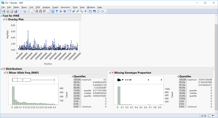
- Individual chromosomes can also be examined by selecting a chromosome of interest from the Tabs section on the left side of the results window. Select Chr 1 Results and Open in New Window. The resulting window has the HWE significance of each marker on chromosome 1 plotted by position as well as distributions for MAF and Missing Genotype Proportion.
- Note that axis settings for the overlay plot can be adjusted by right-clicking the axis on any plot.
- Note that axis settings for the overlay plot can be adjusted by right-clicking the axis on any plot.
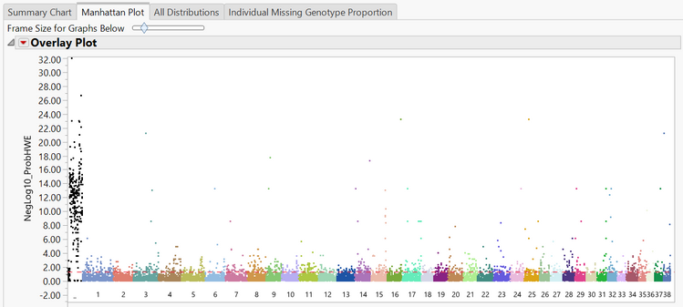
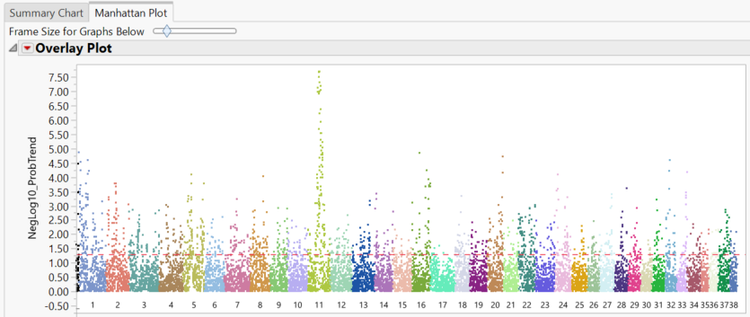
- The Manhattan Plot tab shows a plot of every SNP in the data separated and colored by chromosome number. The y-axis of the Manhattan Plot represents the statistical significance of each marker for Hardy Weinberg Equilibrium. The first chromosome on the plot (colored black) is the X chromosome.
- A subset can be created from the Manhattan Plot by dragging the cursor to highlight a section of SNPs and then and clicking Create Subset Genotype and Annotation Data Sets on the left of the window under the Drill Downs
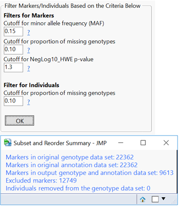
- Note that from the Marker Properties results window, new marker and individual criteria can be set and a new data subset made. The filter tools are located on the left of the window. An example of a re-filtering and its output summary is shown below.
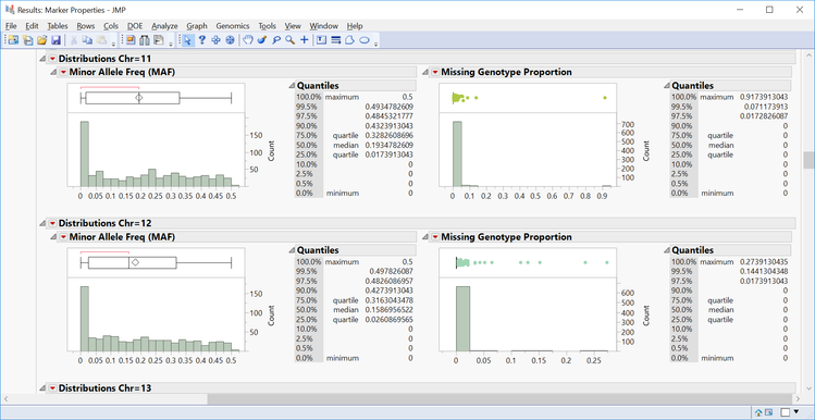
- The All Distributions tab gives distributions for MAF and Missing Genotype Proportion for each chromosome as well as summary statistics of each distribution.
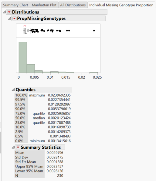
- The Individual Missing Genotype Proportion tab gives a distribution of the proportion of missing genotypes in individuals (rows) as well as summary statistics.
- Return to the journal open the Subset and Reorder Genetic Data results. This is the subset from the criteria specified in the Filtering tab, and removes markers (columns) based on MAF, HWE, and missing genotype proportion. When the results are opened, the summary window will again show which data points have been removed (8,292 markers).
- Return to the journal and open the final output, Case-Control Association. This analysis uses a chi-square test to identify significant markers for the specified trait. The outputted plots are very similar to those from the Marker Properties output, which gives info on HWE.
- Just like the output from Marker Properties, individual chromosomes can be analyzed from the Tabs section, and subsets can be created in the Drill Downs section by highlighting points of interest on the graph.
- Just like the output from Marker Properties, individual chromosomes can be analyzed from the Tabs section, and subsets can be created in the Drill Downs section by highlighting points of interest on the graph.
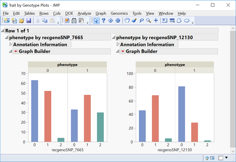
- From the Manhattan Plot tab, drag the cursor around the two of the significant SNPs from chromosome 11 to highlight them. Then select Plot Trait by Genotype from the Drill Downs.This opens a distribution of the genotypes for these two markers by phenotype.
*The interactive reports from this workflow can be viewed on JMP Public.
Summary
Workflows in JMP Genomics are a great way to perform multiple analyses on a single data set. This Basic Genetics Workflow is an effective way to quickly learn the ins and outs of your data, set filtering criteria for both markers and individuals, and get an initial identification of markers of interest. From the Drill Downs menu, there are options for more subsetting, plotting traits by genotype, and exploring linked databases via the gene accession numbers from the annotation data set. This workflow includes a Case-Control Analysis, which is only appropriate for binary traits. For continuous traits, a SNP-Trait association will work (which will be covered later in the series). Now that we have a good understanding of our data, and we have eliminated unwanted rows and columns, we can begin more robust analysis on our subsets.
- © 2024 JMP Statistical Discovery LLC. All Rights Reserved.
- Terms of Use
- Privacy Statement
- About JMP
- JMP Software
- JMP User Community
- Contact



You must be a registered user to add a comment. If you've already registered, sign in. Otherwise, register and sign in.