Genetic Association with JMP Genomics, Part 1: Importing and Cleaning Data

[#1]

In the Genetic Association with JMP Genomics series, we discover numerous methods for associating genetic markers with traits of interest. Before starting any analyses, we need to import and clean our data. In this guide, we download a data set from GEO, bring it into JMP Genomics, and transform it into an ideal form for analysis. In this example, we explore ~22,000 genetic markers in a sample of 474 Bernese Mountain Dogs that are either affected or unaffected for histiocytic sarcomas (tumors).

Importing Experimental Design File

1. To begin, follow the link below to download the xml.tgz data. ftp://ftp.ncbi.nlm.nih.gov/geo/series/GSE38nnn/GSE38011/miniml/
2. Once the files have been saved to your computer, from the Genomics Starter select Import > Experimental Design File > Create Design File from MINiML.
   • The first step in importing the data is creating an Experimental Design File (EDF) from the xml file that was part of the download. This file will contain phenotypic data as well as the file names needed for importing everyone’s marker data.
   • NOTE: The EDF can be created from data in any format by importing into JMP. This includes Excel files and delimited text files which can be accessed through the File > Open command from any JMP Genomics window.
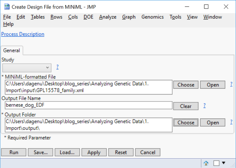
3. On the General tab, select the file xml as the MINiML-formatted File.
4. Type bernese_dog_EDF as the Output File Name and designate an Output Folder, then click Run.
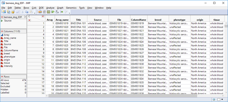
5. The output is an EDF containing the necessary information to import the marker data. Each row in the EDF corresponds to a .txt file containing the marker data each individual dog. The following columns are required in an EDF:

• Array: Unique number for each sample/individual
• File: The name of the file from which to import the sample data
• ColumnName: Unique identifier of each row. Here, each ColumnName entry is the reference ID for a single dog.

Importing Marker Data

6. To import the marker data, return to the Genomics Starter and select Import >Text > Import a Designed Experiment from Text, CSV, or Excel Files.
7. On the General tab, find the EDF sas7bdat and select it as the Experimental Design File.
8. Once the EDF has been designated, click Open next to the file to bring up the EDF table.
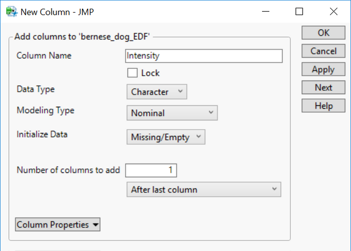
9. At the top of the table select Cols > New Columns.. and create a new column with the Column Name Intensity. Set the Data Type to Character.
10. In the first row of the newly created Intensity column, double-click and enter VAR2.
    • This specifies the second column of each data file as the genotypic data.
    • The column title is designated “Intensity” because an EDF is typically created for expression data.
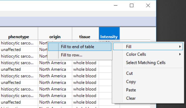
11. Right-click the new cell reading VAR2 and select Fill > Fill to end of table. Once the new column has been created, save the EDF.
12. Returning to the General tab, navigate to the folder where the 476 downloaded files from GEO are stored and designate that folder as the Folder of Raw Files.
13. Select Tab Delimited as the Data File Type.
14. Set the Row Number of Variable Names to 0 and the Data Start Row to 1.
15. Select Use ID Variable as the key variable to merge files and type VAR1 as the ID Variable.
    • This will designate the first column in each file as the ID Variable regardless of its name.
16. Designate an Output Folder.
17. On the Options tab, deselect the option Perform log2 transform. This option is again used for transforming expression data, and does not come into play here.
18. Click Run to begin the process.
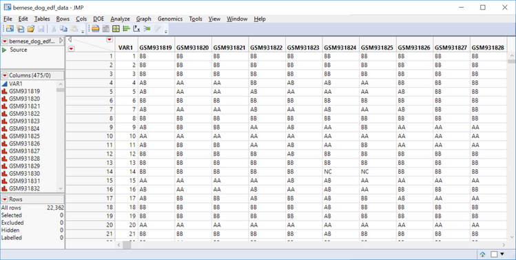
19. The results window will contain a copy of the EDF and a new data set called sas7bdat. Open and inspect the data. Notice it has 475 columns corresponding to individual dogs and markers are organized into rows (tall format).

Transposing Tall to Wide and Combining Data Sets

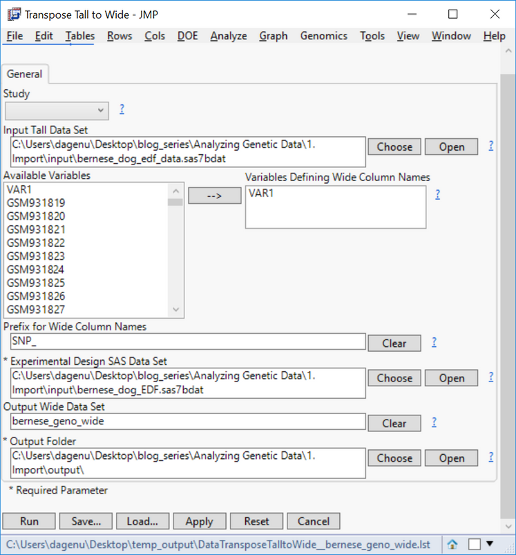
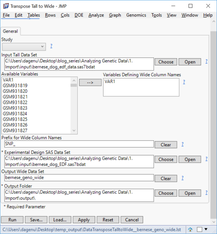
20. The next step is to combine the EDF and the marker data into one wide dataset. Return to the Genomics Starter and select SAS Data Set Utilities > Tables > Transpose Tall to Wide.
    • A wide dataset is necessary to perform most genetics and predictive modeling procedures.
21. On the General tab, choose sas7bdat as the Input Tall Data Set.
22. Select VAR1 as the Variables Defining Wide Column Names, and type SNP_ into the box labeled Prefix for Wide Column Names.
    • This will designate SNP variable names (column names) as SNP_1, SNP_2, SNP_3 etc. in the output dataset.
23. Designate the EDF sas7bdat as the Experimental Design SAS Data Set.
24. Name the Output Wide Data Set bernese_geno_wide.
25. Designate an Output Folder and click Run to begin the analysis.
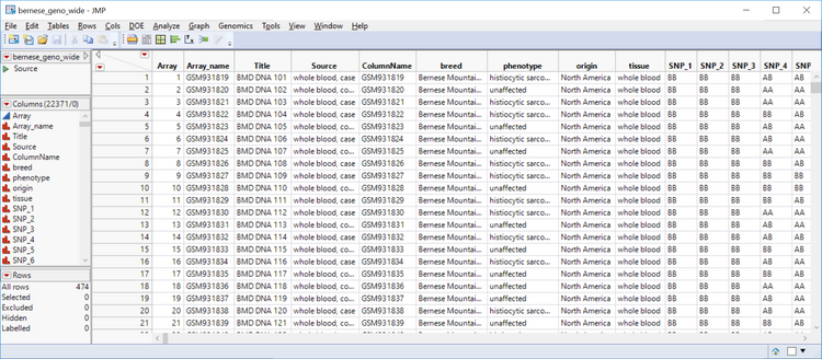
26. Open the output data and inspect it. The result is a wide data set containing both the phenotypic and genotypic data. Notice each genotype is made up of two nondelimited letters.

Recode Missing Genotypes

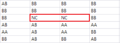
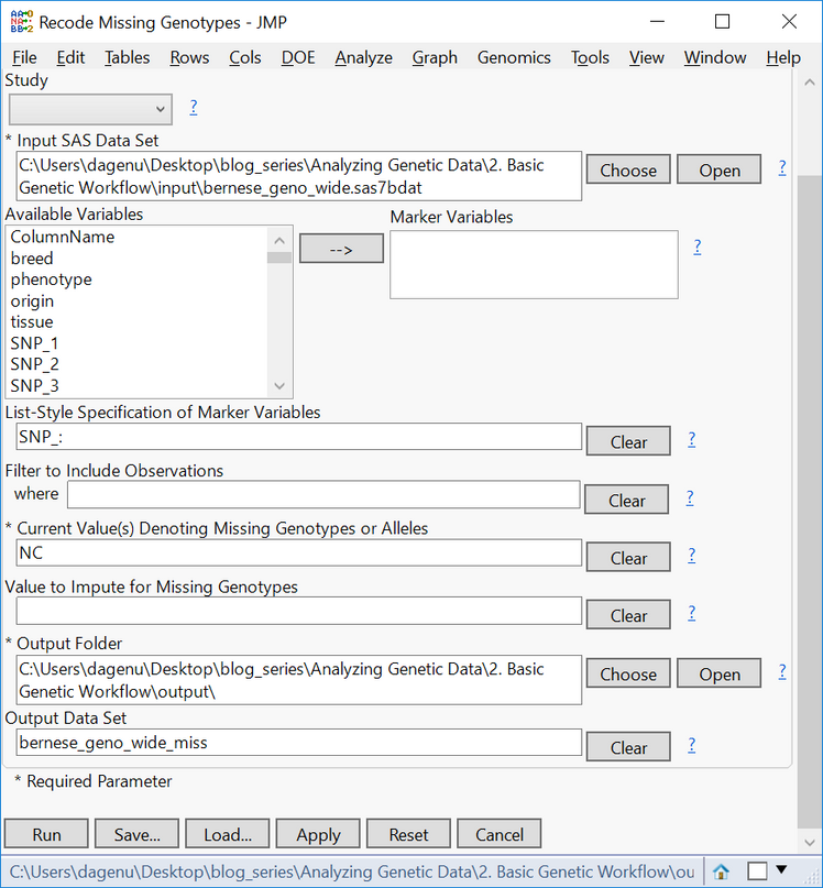
27. The genotypic data in this data set is coded in allele format (AA, AB, BB) with missing data coded as NC. To recode these missing genotypes, return to the Genomics Starter and select Genetics > Genetics Utilities > Recode Missing Genotypes.                       
28. In the General tab, choose the wide data set sas7bdat as the Input SAS Data Set.
29. Type SNP_: into the List-Style Specification of Marker Variables box to specify each column beginning with that character string as a marker variable.
30. In the Current Value Denoting Missing Genotypes box, type NC.
31. Select an Output Folder and name the Output Data Set bernese_geno_wide_miss.
32. Click Run to begin the recode. The resulting data set will have the NC genotypes replaced with a blank cell.

Importing Annotation File (optional)

33. The annotation data set corresponding to these markers is contained in the file GPL15578-tbl-1.txt and can be previewed on the GEO website: (https://www.ncbi.nlm.nih.gov/geo/query/acc.cgi?acc=GPL15578)
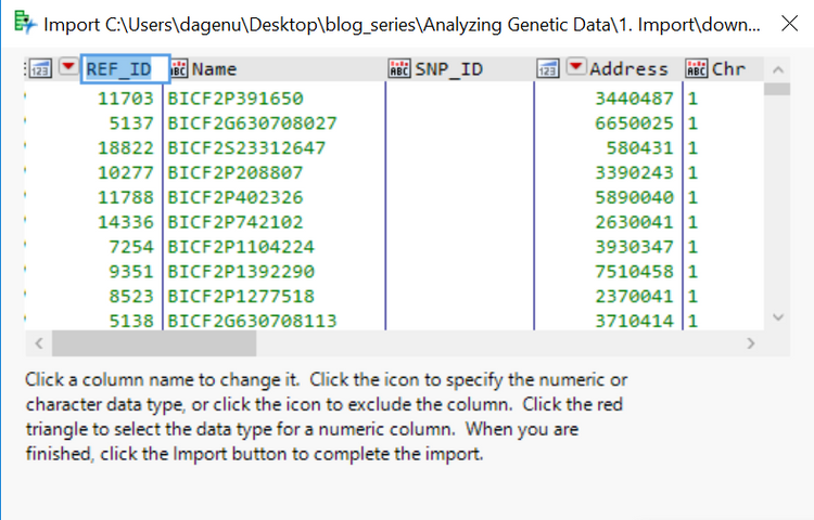
34. A quick preview of the file with a text viewer will show that the file associated with the GEO download does not contain the column names for this data. To solve this problem, they will have to be entered manually. From the Genomics Starter, select File > Open and locate the file GPL15578-tbl-1.txt. Before opening, select the Open as: option Data with Preview. This will open a dialogue box aiding with the import.
35. Select Next to view a preview of the import. From this window, the column names can be changed to match the column names above by simply clicking the column header and typing in the desired name.
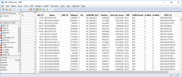
36. Once the column names are entered, click Import to import the data.
37. The first step is to right-click the Name column and select Delete Columns.
    • This column is a duplicate of the SPOT_ID column and can cause problems down the line due to the column name Name.
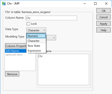
38. Next, right-click the Chr column and select Column Info… Change the Data Type option to Numeric.
    • This will come into play later as the results from some analyses are ordered by chromosome.
39. Right-click on the REF_ID column and choose Sort > Ascending. Once the columns are sorted by REF_ID, right-click the SNP_ID column and choose Formula.
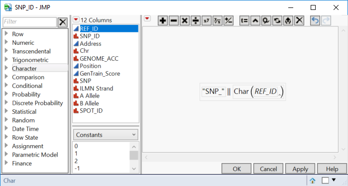
40. In the Formula window, type “SNP_” (including the quotations) into the box. Then from the menu on the far left, select Character > Concat which will add a double bar (||) to the formula. Then, returning to the menu on the far left, select Character > Char and add the column REF_ID to the parentheses. The completed formula should look like the one below.
    • This will take the entries from each row in the REF_ID column and add a prefix “SNP_”. This column will act as the key or reference column for the genotypic data set.
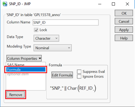
41. Select OK to apply the formula and return to the annotation data set. The SNP_ID column will now be populated. Now, remove the formula by right clicking the SNP_ID column and selecting Column Info…
42. When the window below appears, highlight Formula and select Remove. Then click OK. Note: This should not have any visible effect on the annotation table.
    • Removing the formula allows the column to be unlocked while retaining the information created by the formula.
43. Save the completed annotation data set in .sas7bdat format. Name the file sas7bdat.

Recode to Numeric Genotypes

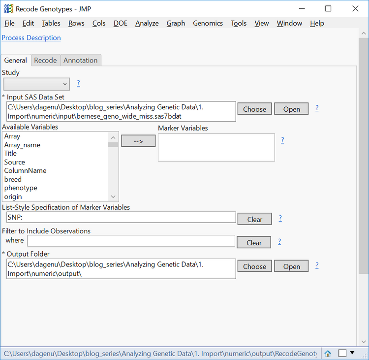
44. The next step will be recoding the genotypes in numeric format. From the Genomics Starter, select Genetics > Genetics Utilities > Recode Genotypes.
45. On the General tab, choose the sas7bdat data as the Input SAS Data Set.
46. Type SNP: into the List-Style Specification of Marker Variables
    • This designates all columns starting with the letters “SNP” as marker variables.
47. Designate an Output Folder.
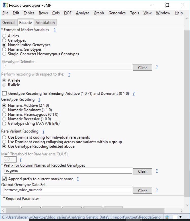
48. On the Recode tab, select Nondelimited Genotypes as the Format of Marker Variables.
49. Leave the default options of Numeric Additive for Genotype Recoding and Rare Variant Recoding.
    • The numeric additive coding is as follows: 0 = homozygous for major allele, 1 = heterozygous, 2 = heterozygous for minor allele.
50. Name the Output Genotype Data Set bernese_wide_numeric.
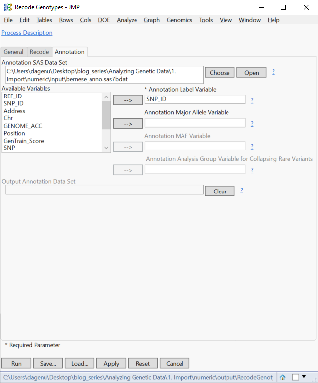
51. From the Annotation tab, select the file from above, sas7bdat as the Annotation SAS Data Set.
52. Enter SNP_ID as the Annotation Label Variable and click Run to begin the recode.
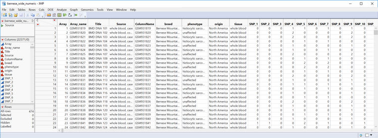
53. Inspect the Recoded genotype data, named bernese_wide_numeric_sas7bdat, from the output window and note the newly recoded genotypes.