- New to JMP? Let the Data Analysis Director guide you through selecting an analysis task, an analysis goal, and a data type. Available now in the JMP Marketplace!
- See how to install JMP Marketplace extensions to customize and enhance JMP.
- Subscribe to RSS Feed
- Mark as New
- Mark as Read
- Bookmark
- Subscribe
- Printer Friendly Page
- Report Inappropriate Content
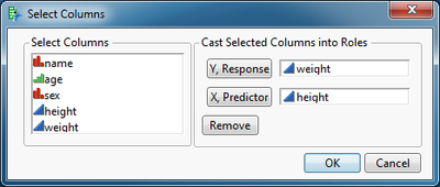
This script creates an interactive demonstration of simple linear regression. You can select data columns for the Y and X roles or you can use a randomly generated data sample. Simply open and run the script:
Select a data column for the dependent variable and click the Y, Response button. Select another data column for the independent variable and click the X, Predictor button. Click OK.
(Note that you do not have to use data columns for this demonstration. Simply click Cancel and the script will generate a random sample for you.)
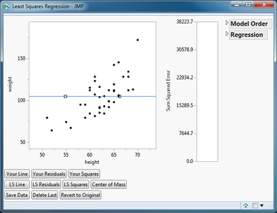
The demonstration provides a scatter plot of the data as its main feature. The horizontal blue line represents your best fit line. It initially represents the null hypothesis that the response is independent of the predictor or that the slope is 0. You fit the blue line to the data by moving it with two handles (small squares). Be careful to place your pointer in the center of the square before dragging it. Also be careful to stop dragging when the square is away from a data point so that it is easy to move it later.
Below the plot is a collection of buttons to turn various graphical features on and off. These features allow you to:
- Add or remove your best fit line, residuals, and residuals squared to the plot.
- Add or remove the least squares best fit line, residuals, and residuals squared to the plot.
- Display a marker for the centroid of the data.
- Save the data to a new data table.
- Delete the last data point.
- Revert the data to the original data set.
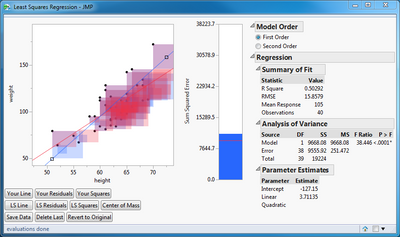
To the right of the scatter plot is a bar chart for the sum of squares of the residuals or error and two outlines. The Model Order outline allows you to alternate between a first-order and a second-order linear regression model. The Regression outline presents the same reports as you would expect from the Bivariate or the Fit Least Squares (Minimal Report) platforms. The Regression outline depends on your line, so if you move the line, this report is immediately updated.
A typical demonstration might follow these steps:
- Fit your line by dragging the two handles.
- Click Your Residuals to add the vertical lines representing the regression errors. (Also represents visual criterion used by the human eye - balance the errors on both sides of the line.)
- Click Your Squares to add the shaded square representing the squared regression errors. This action also activates the bar chart to the right of the scatter plot. (Represents the actual criterion used by least squares regression for the best fit line. Area is not easily discernible by the human eye.)
- Click LS Line to add the line representing the least squares regression for comparison.
- Click the LS Squares to add the shaded square representing the squared regression error. This action also adds a reference line to the bar chart.
Further possibilities include changing the data. You can drag a data point. You can click anywhere to add another data point. These features allow you to discuss leverage (move a data point vertically (change in response) for an observation near the center or near one of the ends) and influence (change the scale of the axes and add a new observation far away from the original data and out of line with the regression fit).
Recommended Articles
- © 2026 JMP Statistical Discovery LLC. All Rights Reserved.
- Terms of Use
- Privacy Statement
- Contact Us


