- Subscribe to RSS Feed
- Mark as New
- Mark as Read
- Bookmark
- Subscribe
- Printer Friendly Page
- Report Inappropriate Content
JMP Add-Ins
Download and share JMP add-ins- JMP User Community
- :
- File Exchange
- :
- JMP Add-Ins
- :
- Compare Simple Slopes in One-Way ANCOVA (w Interaction) add-in
This add-in ingests estimates from a Fit Model report of a one-way ANCOVA with interaction to generate a combined data table of indicator parameterization estimates treating each level of the categorical variable as the reference category successively. This allows for testing of pairwise slopes in this analysis.
Instructions (after installing add-in):
- Fit an ANCOVA with interaction model using Fit Model
- Select Add-ins > One Way ANCOVA with Interaction Simple Slopes Test
- A combined data table of indicator parameterized estimates will be produced treating each level of the categorical X as the reference
- Parameter estimates for lower order terms and their associated t-ratios and p-values indicate a test of mean difference on Y at the mean of the continuous X for that term vs. the reference category
- Parameter estimates for the interaction terms and their associated t-ratios and p-values indicate a test of the difference in slope of Y against the continuous X for that term vs. the slope of Y against the continuous X for the reference category
- Parameter estimates for the continuous X and their associated t-ratios and p-values indicate a test of the slope of Y against the continuous X for the reference category against 0 (this is also where you look to see the slope of each category)
Expanded details and example:
An ANCOVA including an interaction is a type of multiple regression in which one continuous Y is modeled by one categorical X, one continuous X, and the interaction between the two. A traditional ANCOVA does not include this interaction (and a critical assumption is the homogeneity of regression) but sometimes it is the case that there is evidence the slopes between Y and the continuous X differ across the levels of the categorical X (e.g. a statistically significant interaction or prior theory predict this). When there are 3 or more levels of the categorical predictor, it's useful to follow-up on this interaction with pairwise tests of slopes to see for which groups the slopes differ. In the example below I'll use the US Demographics sample data table available in the sample data directory.
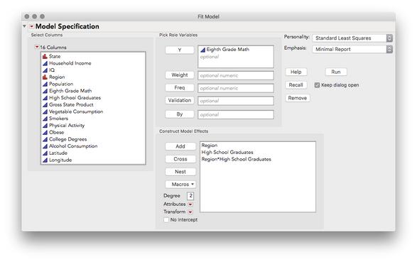
First, let's fit a model using Analyze > Fit Model. Here I will predict Eighth Grade Math (continuous) on the basis of Region (nominal), High School Graduates (continuous), and the interaction of the two. This is the only structure this add-in currently supports (i.e. continuous ~ nominal + continuous + nominal*continuous)
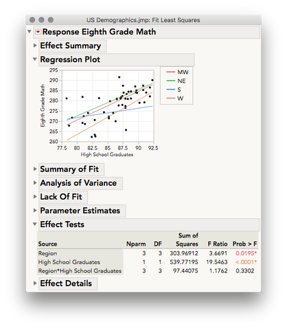
In the regression plot we see regression lines for Eighth Grade Math against High School Graduates for each region.
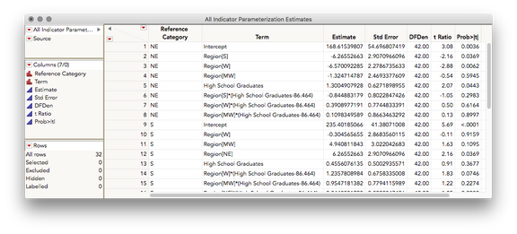
Several of these regions appear to have a similar regression, but the slope of the south appears to be a bit different. Our overall effect test for Region*High School Graduates does not give us substantial evidence there is an interaction (p = 0.3302) so we might simply regard this difference in slope for the south to be random error. For this example, let's follow-up on these slopes anyway and produce pairwise tests of the slopes. To do this, run the add-in, Add-ins > One Way ANCOVA with Interaction Simple Slopes Test. This will produce the table of estimates below:
This table was constructed by requesting indicator parameter estimates for this model (estimates that reflect deviations from a reference category) treating each region as the reference. The Reference Category column indicates which level of Region is used as the reference for each row.
There are four types of estimates in this table:
- Intercept: this is the Y-Intercept for the regression of Y on to the continuous X for the listed reference category. For example, in row 1 NE is the reference category. So, 168.615 is the Y-Intercept for the regression of Eighth Grade Math against High School Graduates for just the NE
- Region[] : Each of the Region[] terms are estimates for the mean difference in Eighth Grade Math for the listed region against the reference region, assuming an average value for High School Graduates. For example, in row 2 Region, and the estimate -6.266 indicates that the Southern region had a mean score on Eighth Grade Math that is 6.266 points lower than the NE (the reference category), assuming they both had an average amount of High School Graduates. Note: this emphasis on the "average amount" of the continuous X is due to the fact that this is a centered model. Since the slopes between Y and the continuous X may differ, we need to speak about mean differences between groups at a certain level of the continuous X. In a centered model, that location is the mean of the continuous X.
- High School Graduates: This is the slope for the regression of Y on to the continuous X for the listed reference category. For example, in row 5 NE is the reference category. So, 1.300 is the slope for the regression of Eighth Grade Math against High School Graduates for the NE
- Region[]*(High School Graduates - mean): Each interaction term indicates the difference in slope of Y against the continuous X for that term vs. the slope of Y against the continuous X for the reference category. For example, in row 6, Region *(High School Graduates-86.464), the estimate -0.845 indicates that the slope of Eighth Grade Math against High School Graduates for the South is 0.845 points lower than the slope of Eighth Grade Math against High School Graduates for the NE (the reference category). Note: the constant that is being subtracted from High School Graduates is the mean level of high school graduates across all groups. This is what makes this a centered model).
- T-ratios and p-values associated with each row may be used as tests for any estimate. For example, if we wish to test the difference in slope of Eighth Grade Math against High School Graduates for the South vs the West, we could look in row 14, Region*(High School Graduates-86.464) with the reference category listed as the South. We find a difference in slopes of 1.236 points, t = 1.83, p = 0.0746. By a standard of alpha = 0.05 we would fail to reject the null hypothesis; we can only conclude that we do not have sufficient evidence to regard these slopes as different.
- Notice the same information for the above test is provided in row 24, Region *(High School Graduates-86.464), with the West listed as the reference category. Only the sign of the difference has changed.
Revision History:
v0.02 - Added support dialog to select from multiple least squares reports
v0.03, v0.04 - Fixed defect: script failed when nominal column was numeric
v0.05 - Fixed defect: when partial value ordering was set additional levels were ignored.
Hi,
I tried running this add in and it didn't give any new table of results.
Looking at the Log i found that an error is in the line
reDoScript = Get Clipboard() /*###*/;
what could be the problem?
Thanks, Eli
Hello,
Very useful addin, thank you very much!
I have a question concerning the p-values. I know that for some tests performed in JMP, the p-values are corrected for multiple comparaisons. Is this the case here?
Also, is the test still valid for a situation in which the categorical variable would be Y and not X (opposite to what's explained in the expanded details)?
Thank you,
Andreea
Hi- I am getting the error "could not find column in access or evaluation of 'Column' , Column/*###*/(nomName)". Any thoughts on how to troublehsoot?
Thanks!
Laura
Recommended Articles
- © 2026 JMP Statistical Discovery LLC. All Rights Reserved.
- Terms of Use
- Privacy Statement
- Contact Us


