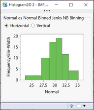
This Add-In draws histograms with varying base widths of the bins that subdivide a continuous variable's x axis. The width of the bins can be derived from the data itself or from a binning formula. In 2D-histograms the area over the bin represents the number of observations within, not the height of the bar. The height of a bar is the density of observations over the base.

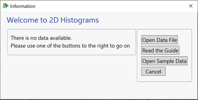
Picture 1: Information Window
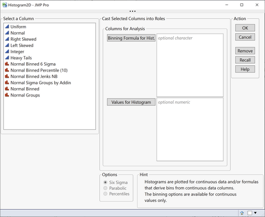
The Add-In first tests if a data set is available. If not, a window informs the user and asks for some action (Picture 1 ). If a data table is open, the “platform” dialog (Picture 2 ) is shown.

Picture 2: Addin Dialog
You are familiar with the column list on the left from all the other JMP dialogs. The role frame contains two target areas, the first one for formula columns the second for continuous variables.
Binning Formula for Hist.


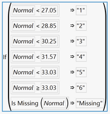
Picture 3: Binning Formula Picture 4: 2D Histogram
Binning formulae subdivide the range of continuous variables into sections, called bins. These formulae are a sequence of nested If-Then-Else statements, like the one in Picture 3 . They reference a data column, “Normal” in this case, and provide a list of cut-points that split the axis into the bins. These binning formula columns are always categorical. The Add-In extracts the variable name and the cut-points from a formula and uses both to calculate densities and plot the histogram. There are many ways to set up formulae for binning. This Add-In extracts the necessary information from formulae that are derived from the Binning Add-In V2 or, from the column utility for binning built in JMP. When using the column utility from JMP then the “Bin Label” from the hot spot MUST BE “Character”. Otherwise the bins can not (yet) be derived. If you want to set up your own binning formula and show the result with 2D Histogram, you should build the formula pretty much the same way, otherwise the Add-In may have trouble isolating the right elements. The histogram derived from the formula in Picture 3 is shown in Picture 4 . Note that the bins are wider in the tails than in the center.
Values for Histogram
Continuous variables can directly be plotted in a 2D-histogram. For the purpose of binning there are three options available. The selected option is applied to all variables in the “Values for Histogram” list. The option “Six Sigma” calculates mean and standard deviation from the data, sets up the bins in 1-sigma steps and centers them around the mean. All data outside the six-sigma range is collected in one or two “remainder” bins which stretch out to cover the minimum and/or maximum.
The "Parabolic" option tries to find the empirical mode of the data and makes the bins larger the farther they are away from the mode. The increase of the bin widths follows a parabolic growth.
The "Percentiles" option searches for a percentage that is a compromise between sparsity of the bins and detail of the distribution. For this percentile the binning is made. Percentile binning makes intervals with (almost) identical numbers of observations.
For every option a set of statistics is printed and a reference value is added to the x-axis, if appropriate.