
The K Nearest Neighbours, or KNN, platform predicts a response value for a given observation using the responses of the observations in that observation’s local neighbourhood. It can be used to classify a categorical response as well as to predict a continuous response.
KNN is a non-parametric, supervised machine learning algorithm. It works on the underlying assumption that similarities in certain parameters (the observations) reflect similarities in other parameters (the prediction). To fulfil this assumption, KNN ranks the k smallest distances between the given observation and all other observations.
Because of this fact, K-Nearest Neighbours can classify observations with irregular prediction boundaries. However, as the algorithm is sensitive to irrelevant predictors, the choice of predictors can affect your results.
Calculate the distance
JMP pro 17 uses Euclidean Distances to calculate the distances between the predictor values and those of others. In a 2D space, the Euclidean Distance d between (x1, y1) and (x2, y2) is simply:
d = sqrt((x2-x1)^2 + (y2-y1)^2)
the Euclidean method requires that all the values are real.
Making predictions
The KNN gives its prediction depending on the types of responses it has.
- Continuous responses
JMP predicts values as the average of the responses of the k nearest neighbours. Each continuous predictor is scaled by its standard deviation. Missing values for a continuous predictor are replaced by the mean of that predictor.
- Categorical responses
In JMP, the predicted value is the most frequent response level for the k nearest neighbours. If there is more than one top response, the predicted response is assigned by randomly selecting one of these levels.
The k value or n_neighbors
Different values of k can give different predictions. In JMP, you only need to specify the maximum number of k. For each k, 1 ≤ k ≤ k_max, JMP builds a model using only the training set observations. Each of these models is used to classify the validation set observations. The validation set results are used to select the model with the lowest misclassification rate (aka the best k).
Validation for KNN in JMP modelling
You can add a numerical column as a validation for KNN modelling in JMP Pro. JMP uses validation to partition data into sets before modelling to reduce overfitting and select a good predictive model. For KNN, this feature is optional. However, overfitting can lead to a mismatch between training and prediction, i.e., the algorithm is overly specific to the training data, resulting in less accurate predictions.
For KNN, you can partition the data into two or three sets by the following methods:
|
Method
|
Set
|
Function
|
|
Train and tune
|
Training
|
Estimate model parameters
|
|
Validation
|
Tune the model parameters in the model fitting algorithm, and ultimately choose a model with good predictive ability
|
|
Train, tune, and evaluate
|
Training
|
Estimate the model parameters
|
|
Validation
|
Tune the model parameters in the model fitting algorithm, and ultimately choose a model with good predictive ability
|
|
Test
|
Independently evaluate the performance of the fitted model
|
Learn more about validation in the JMP Documentary: Example of the Make Validation Column Platform (jmp.com)
Example
In this example, we want to use KNN to categorise a customer between Good Risk and Bad Risk based on their financial history.
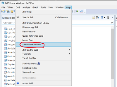
- Select Help > Sample Data Folder and open Equity.jmp.
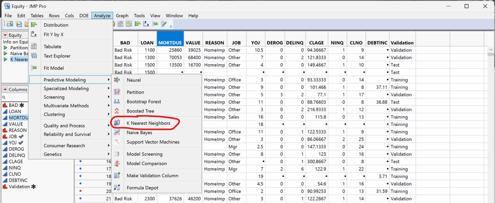
- Select Analyze > Predictive Modeling > K Nearest Neighbors.
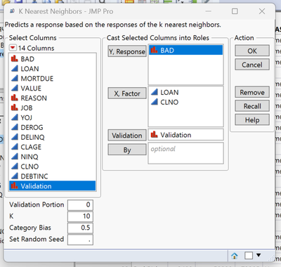
- Select BAD and click Y, Response. The is the value to analysis.
- Select LOAN and CLNO and click X, Factor. This is the predictor variables.
- Select Validation and click Validation. This is the value used to partition data into sets before modelling to avoid overfitting and select a good predictive model. We used Train, Tune, and Evaluate method in the example.
- Click OK.
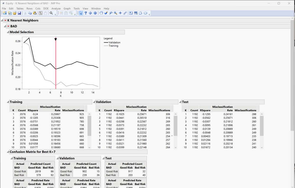
To save the prediction equation
- Right click the BAD red triangle and select Publish Prediction Formula.
- Next to Number of Neighbors, K, leave the default value of 7.
- Click OK.
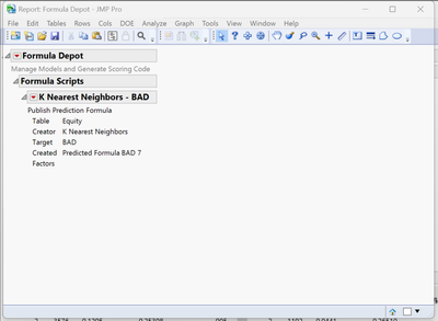
The prediction equation is saved in the Formula Depot. You can compare the performance of alternative models published to the Formula Depot with that of the K = 7 nearest neighbour model using the Model Comparison option in the Formula Depot. Find more information regarding the Formula Depot in Help/JMP Documentation Library, page 3763.
If you are interested, you can go back to the step 4. This time put all the parameters in between LOAN and CLNO as X, Factor. What changed and why?
Shuran,
Reviewed by Jeremy T. @Jeremy_Tee
Jan 2024, Based on JMP(R) Pro 17.2.0
This article does not reflect the positions and opinions of JMP Statistical Discovery nor SAS Institute.