Calculating Full Width at 0.01 (FW(0.01)) for Detected Peaks

[#1]

I have time series data (attached) representing concentration over time, and I want to apply a Savitzky-Golay smoothing first and then detect peaks in JMP. While I know how to perform the peak detection, I’m struggling with how to calculate the Full Width at 0.01 (FW(0.01)) for the identified peak.

Here’s my plan to do it manually thus:

1. Locate the Peak: Identify the maximum value of the peak (here 826163 in my table) 

2. Determine the 0.01 Threshold: Calculate the value that corresponds to 1% of this height by multiplying the peak height by 0.01 (826163  * 0.01 = 8261.63 in my table).

3. Identify Points at the 0.01 Threshold: Find the x-values where the signal intersects this threshold on both sides of the peak (HERE IS MY PROBLEM)

4. Calculate FW(0.01): Once I have the two x-values (x1 and x2) where the signal crosses the 0.01 threshold, calculate the full width as:

   • FW(0.01) = x2 - x1.

However, I’m unsure how to effectively recover the intersection points  with the threshold in my smoothed data: X1 and X2. I could use a dichotomous method or interpolation, but I'm looking for a more straightforward/precise approach. Is there any way to do it using Profiler, Invert Smoothing or another method ?

[#2]

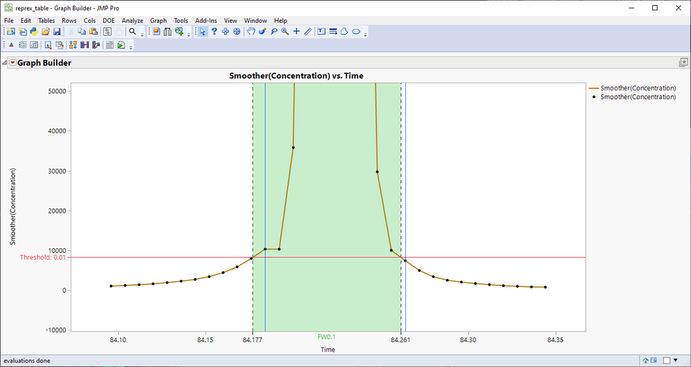
I will go with the assumption that you will have lines between each of the markers (based on the graph found from table)

Names Default To Here(1);

dt = Open("$DOWNLOADS/reprex_table.jmp");

m = dt[0, "Smoother(Concentration)"];
peak = Max(m);
threshold = 0.01*peak;

low = Min(Loc(m > threshold));
high = Min(Loc(m[low + 1::N Rows(m)] < threshold) + low);

low_c = m[low-1::low];
low_t = dt[low-1::low, "Time"];
low_i = Interpolate(threshold, low_c, low_t);

high_c = m[high-1::high];
high_t = dt[high-1::high, "Time"];
high_i = Interpolate(threshold, Reverse(high_c), Reverse(high_t));

Show(high_i, low_i);

// Just for visualization
gb = dt << Graph Builder(
	Size(528, 454),
	Show Control Panel(0),
	Variables(X(:Time), Y(:"Smoother(Concentration)"n)),
	Elements(Line(X, Y, Legend(6)), Points(X, Y, Legend(7)))
);
rep = Report(gb);

rep[Framebox(1)] << Add Graphics Script(
	Pen Color("Red");
	Pen Size(1);
	H Line(threshold);
	
	Pen Color("Blue");
	V Line(dt[low, "Time"]);
	V Line(dt[high, "Time"]);
);

Eval(EvalExpr(
	rep[AxisBox(1)] << Add Ref Line(
		Expr(low_i),
		"Dashed",
		"Black",
		Expr(Char(Round(low_i, 3))),
		1,
		1
	)
));

Eval(EvalExpr(
	rep[AxisBox(1)] << Add Ref Line(
		Expr(high_i),
		"Dashed",
		"Black",
		Expr(Char(Round(high_i, 3))),
		1,
		1
	)
));

Eval(EvalExpr(
	rep[AxisBox(1)] << Add Ref Line(
		{Expr(low_i), Expr(high_i)},
		"Solid",
		"Green",
		"FW0.1",
		1,
		0.25;
	)
));

Write();