- JMP User Community
- :
- JMP Discovery Summit Series
- :
- Past Discovery Summits
- :
- Discovery Summit Europe 2019 Presentations
- :
- The What, Where, Why and How of Functional Data Explorer ( 2019-EU-45MP-050 )
- Subscribe to RSS Feed
- Mark as New
- Mark as Read
- Bookmark
- Subscribe
- Printer Friendly Page
- Report Inappropriate Content
Level: Intermediate
Job Function: Analyst / Scientist / Engineer
Peter Hersh, JMP Senior Systems Engineer, SAS
One of the marquee features in JMP Pro 14 is the Functional Data Explorer (FDE). But what is "functional data" and how exactly do we "explore" it? Functional data is everywhere. It takes the form of sensor data, transactional data, chemical spectra – the list goes on. The common thread is that it can be challenging to analyze. Moreover, we generally don't want to analyze the functional data directly; we want to work with the underlying information – the functions that are producing the observed data. The FDE helps us do this. It serves as a tool for both exploratory analysis and dimension reduction to help us use the functional information in other modeling techniques. In this presentation, I will show the new analytical problems JMP can answer using FDE through several case studies from industrial, chemometric and the financial domains. Along the way, I will demonstrate FDE and some of the tips and tricks learned while helping customers understand how powerful this new platform truly is.
Functional Data explorer was introduced in JMP Pro Version 14 and enhanced in Version 14.1.
This paper describes how to perform functional data analysis in JMP Pro 14.2 utilizing Functional Data Explorer.
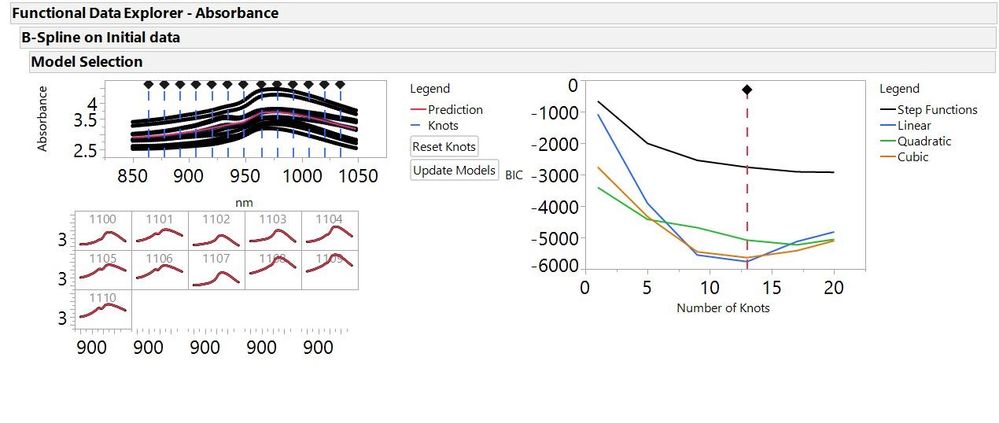
Figure 1. A Snapshot of Functional Data Explorer Fitting a B-Spline Model to Absorbance Data
History
The term Functional Data Analysis was first coined in 1982 by Ramsay, but has a history dating back to Grenander in 1950. The idea is to treat data as a continuum instead of discrete measurements. This is accomplished by creating a function to describe the data.
How to Use It
Launching Functional Data Explorer
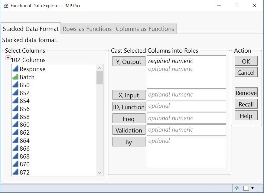
To utilize functional data explorer, you must have JMP 14 Pro or more recent version of JMP Pro. Functional data explorer is found under the analyze menu specialized modeling. There are 3 options for data format stacked in rows or in columns. Stacked data format is preferable allowing tha analyst to look at several functional responses at once.
Figure 2. Functional data explorer launch window
Data Processing in the functional data explorer
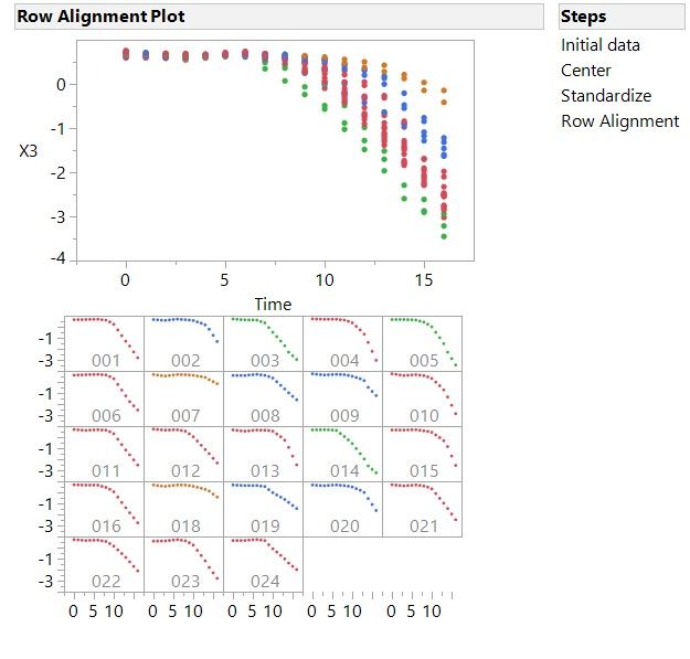
After launching functional data explorer, the data processing window shows up this allows you to perform many different process to clean the data. There are 3 types of data processing found in functional data explorer; cleanup, transform and align. Cleanup allows you to remove points that are not helping define the continuum of points these can be zeros, specific values or outliers. Transform allows you to quickly transform your response y-variable to center (set mean to 0), standardize (set standard deviation to 1) or stabilize variance. Align enabls you to align the x-variable either lining up minimum, row, maximum or align to a reference function using dynamic time warping. Dynamic time warping uses a reference spectrum and reduces the y residual of the original spectra to the reference spectra. It accomplishes this by aligning the x-values in the original data to the reference spectra that has the most similar y value. All data processing steps are recorded in by the data processing steps and can by removed.
Figure 3. Data Processing window
After processing is complete the data can be saved by going to the red triangle and selecting save data. This will allow you to create a new cleaned up data table.
Model fitting
Once the data has been cleaned up you can now fit a model to the data. The model fitting can be found under the red triangle and models. In JMP Pro 14 there are 3 options for model fitting, B-splines, P-splines and Fourier basis. B-splines are a piecewise polynomial model where the number of pieces (Knots) and the degree of polynomial can be defined (degree = 0, 1, 2, or 3). P-splines are a penalized version of B-splines. Fourier basis models are built using sine and cosine functions of increasing periodicity. Fourier basis models work well with periodic data. When you run the model JMP will automatically run a group of models and select the model that best fits your data using a specified information criterion (BIC, AICc or GCV). You can adjust the number and location of knots as well as the degree polynomial of the fit.
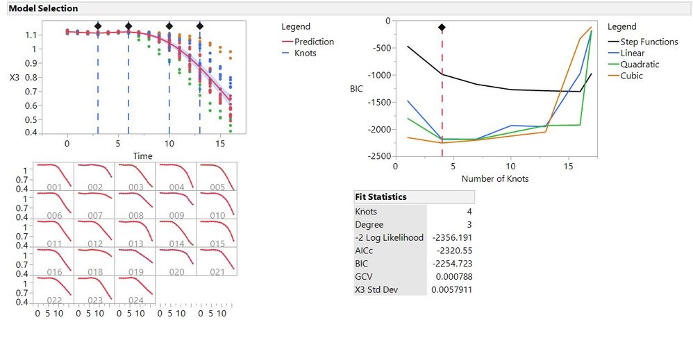
Figure 4. Model selection from FDE showing a 4 knot cubic fit as the best model selected by BIC criterion
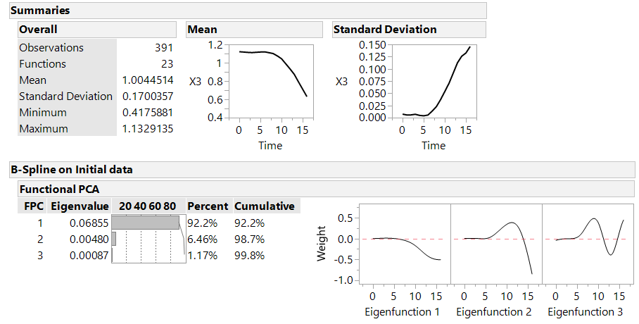
In this example we have 4 knots meaning that we have 5 separate polynomial models (cubic in this case) that fit the data between each knot. Once your piecewise polynomial model is finalized functional principle components (FPCs) will be generated to define the function. JMP will generate all the FPCs that define at least 1% of the overall variance. The these FPCs define the shape variation from the mean. Each batch is assigned a value for each FPC. If your data tracks the mean function exactly all the FPCs would be 0. If you have a positive value FPC the shape of the function varies from the mean in a similar shape to the corresponding eigenfunction (negative FPC indicates the reverse effect).
Figure 5. Example of the Mean Function and the variations to that mean function called eigenfunctions.
Saving your Functional Principle Components
Once the model has been completed and fit to your data a functional summaries table is created. This gives functional principle components for each batch of your data. You can customize which summaries you would like and how money FPCs you would like to have generated. Then this table can be saved and used for data analysis.
Example 1 DoE Response for Tablet Dissolution
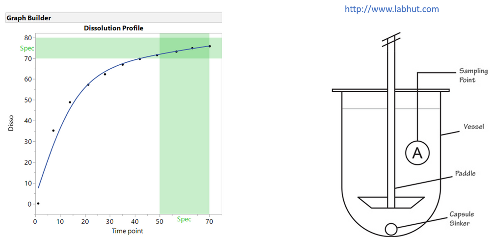
In the pharmaceutical industry, drug dissolution testing is used to provide critical drug release profiles for oral dosage. This testing is critical for both drug development and assessing batch to batch variability. The test is designed to be a surrogate for human studies and is regulated by the Food and Drug Administration (FDA). Analytical data from drug dissolution testing are often used to establish safety and efficacy of a drug product. In this example we are trying to optimize a dissolution profile to hit our spec window. Typically dissolution testing is measured at different time points to establish a profile. In this example we have a specification of 70-80% dissolution and we want that spec to be maintained throughout 50-70 minute range. This example will use functional data explorer to examine the data and come up with the ideal setting to get a profile that meets specs and is robust.
Figure 6. Quick view of dissolution process and profile
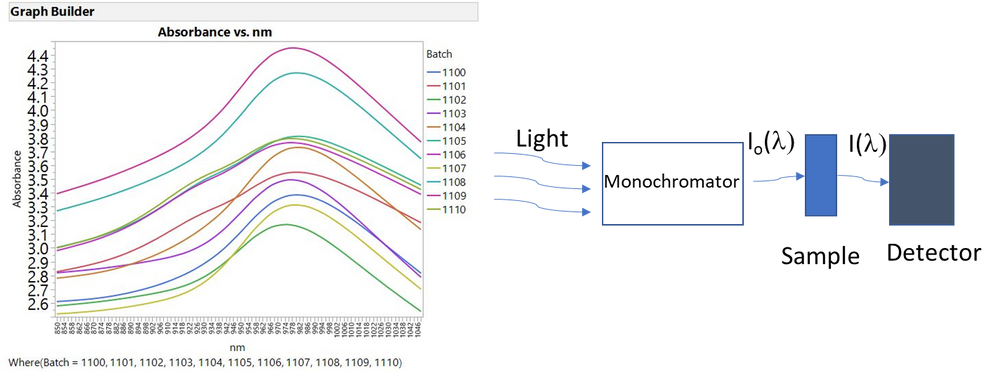
Using functional data explorer to examine in spectral data. In this example we are using near IR radiation to look at fat content in beef. This is in place of a destructive technique for determining fat content
Figure 7. Spectral information from fat content in beef study
Example 3 Enzyme Yield from Fermentation Process
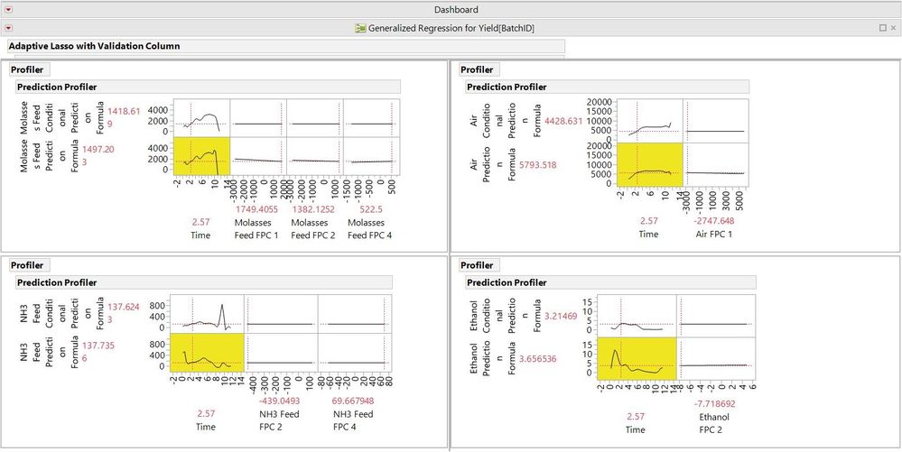
Looking at shape of a group of input variables to make a predictive model of yield. Identifying what the ideal shape for each input variable will be to maximize yield.
Figure 8. Yield Dashboard
Summary
Functional data can be found in many various places across different fields and applications. Often, we are not taking full advantage of the functional data by summarizing the data. This throws out a substantial portion of the collected data and does not allow us to capture all the potential information. Functional data explorer in JMP 14 Pro helps us capture all of the information by using functional principle components to capture the shape of the functional data.
References
“Ramsay JO. 1982. When the data are functions. Psychometrika 47:379–396”
Grenander U. 1950. Stochastic processes and statistical inference. Arkiv f¨or Matematik 1:195–277
- © 2024 JMP Statistical Discovery LLC. All Rights Reserved.
- Terms of Use
- Privacy Statement
- About JMP
- JMP Software
- JMP User Community
- Contact
