Level: Beginner
Daniel Valente, PhD, JMP Senior Product Manager, SAS
Jon Weisz, JMP Senior Vice President Sales and Marketing, SAS
Abstract
Often, JMP users have experienced an interactive JMP session that left them with many windows and analyses reports opened all at once. While using JMP in this "floating-window mode" may work for some, there are situations where having a tabbed interface is preferred. Users also may want to associate certain files with an analysis project and not have the full list afforded by the Home Window. For these reasons, we created projects in JMP 14. Projects provide a single document interface to JMP, a tabbed, re-configurable work space, a place to bookmark files and a window list that lets the user easily navigate various open windows, data tables, scripts and more; it also launches supporting files like .pdfs and .ppt documents. Projects can be used to quickly open and close many files associated with one or more individual analysis activities and can be used to keep parallel projects separate, eliminating the need to run multiple JMP sessions. Finally, projects in JMP 14 can also give you an easy way to share and collaborate on work with their archiving functionality.
Overview of JMP Projects
Projects in JMP are a way of organizing data tables, reports, scripts, journals and artifacts of using JMP in JMP. You can also associate external supporting files such as .txt, .ppt, .html, .xls and images with the appropriate project files associated with a logical group of native JMP files.
The project file itself (.jmpprj) is a standalone file, which points to other items on your disc, rather than acting as a container in which to put files. As a result, this affords the flexibility and organizational discipline of a container-based project, while at the same time keeping the files available to be found on the operating system.
JMP projects are created from the File menu (File > New Project). The creation of a new project will immediately open an unsaved project in which to add JMP windows and files, making it easy to create temporary projects.
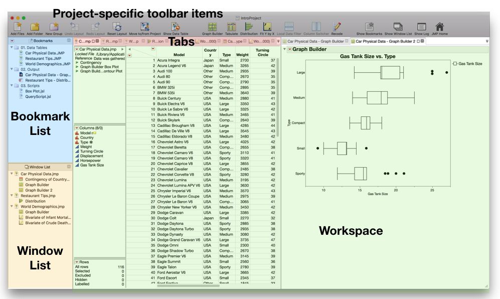
An example of a JMP project is shown in Figure 1. A project includes three major sections:
- Bookmarks List: Links to physical files on disk that you want to associate with the project. This is like a curated list from the Home Window. Bookmarks can be links to individual files, links to folders (which automatically “watch” what is inside, including subfolders), and groups, providing local organization specific to files in the project without affecting the folder structure of the files on disk.
- Window List: Hierarchical list of open data tables and reports and graphs associated with the data table.
- Workspace: Tabbed list of windows, including scripts, graphs, model output and data tables currently open in-memory. The layout can be arranged from a single column of tabs (e.g., like a Web browser) or arranged into columns of tabbed lists. The layout is persisted when a project is opened and stored when it is closed.
Figure 1: A sample JMP project with annotated major sections.
For example, projects can be used for:
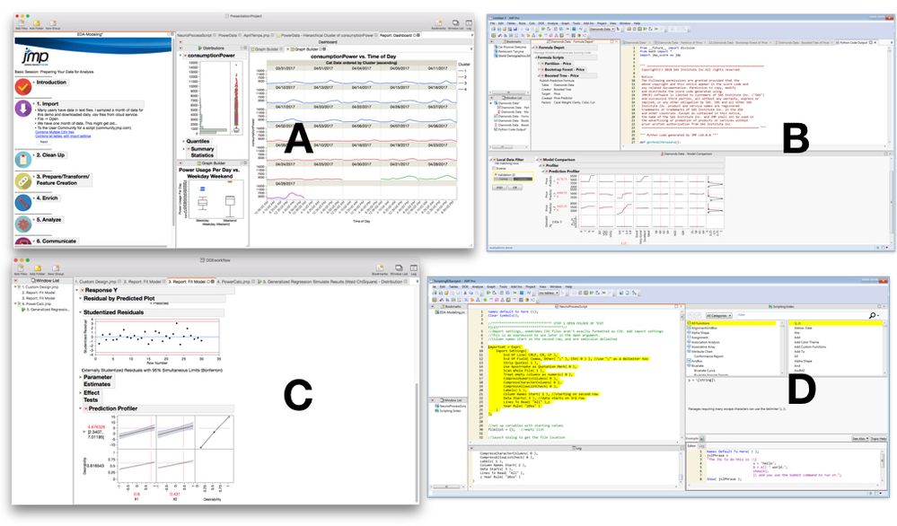
- Presentation of results. This project is shown in Figure 2A. The project has been configured to hide the bookmark and window lists. There is a column with a single tab, which has a journal running the presentation. The journal includes links to scripts and support files, which, when clicked, show up in the projects as tabs. The journal affords the ability to add notes and context to the rest of the items in the project.
- Predictive modeling workflow. This project is shown in Figure 2B and will be covered in the Case Study II later in this paper. The project including performing standard predictive modeling tasks on a single data set. Multiple models are fit and saved to a Formula Depot as they are built. The Formula Depot is in its own column so it can easily be referenced. Finally, a Model Comparison is added and score code is generated for putting the model into production.
- DOE workflow. This project is shown in Figure 2C and a DOE workflow like this will be covered in Case Study I later in this paper. The project is used for organizing the steps for creating a designed experiment, comparing multiple candidate designs, collecting data, analyzing data and creating output for sharing results with others. It can also include supporting materials about the experiment (photos, reports, etc.).
- Scripting project. This project is shown in Figure 2D. It is used to help JSL scripters organize their windows and make it easier to be efficient while scripting. The project includes the scripting index in a mode configured specifically for use in a project. The script being worked on includes an embedded log and also links to supporting files or functions in the bookmark list.
Figure 2: Ways that projects can be used in JMP.
Who is the Intended User of JMP Projects?
Projects are an optional way of working in JMP and many users will continue to operate in the standard “multiple-window mode” of JMP. However for those who work in JMP in a specific way or have specific pains around window management or file management, the project is worth checking out.
Many users prefer to run JMP platforms such as Graph Builder with a maximized window. Unfortunately, once a window in JMP is maximized, it is easy for new users to lose the data table or to have difficulty navigating to other windows currently open. By utilizing a tabbed workspace, the project gets around many of these pains. A user can simply navigate to another open tab, like when using a Web browser, to get to another analysis report or data table.
For folks who have standard weekly or daily reports, the project can be an efficient container to support that work. Coupled with the Query Builder, for example, a project can include a script that fetches the most recent data from a database and generates a set of standard reports; it can then be saved with the date to streamline this routine reporting task.
Long-time JMP users may remember (and miss) the Master Window on the Windows version of JMP. Now with the project, they can restore much of that functionality.
For users who generate many windows – either interactively or through scripting – and feel as though they get lost in a session, the project can help ease this pain. When a user is working on multiple projects at once, closing a single project can automatically close all the files and windows associated with that project, while leaving the other projects untouched and eliminating the need to manually close multiple windows.
For users who have already worked out their own file organization scheme for JMP output and files, projects can provide a framework or fit well within a folder-structured way of using JMP. And finally, people who have files all over their computer’s hard drive can add individual files to a project to pan an organized structure on top of a messy folder.
Working with the Project
Getting Files into a Project
First start by creating a new project (File > New Project). Files can be added to a project individually by Adding Files. Files added to the project get added to the Bookmarks list. When files are added individually, it can be useful to create a group, local to the project, which can further organize your bookmarks. Create a group by running the New Group command and then renaming the group to something descriptive.
- Pro Tip: Groups can be used to set up template projects to make it easier to get up and running when a new project is needed. Groups such as “Data Sets,” “Reference Scripts,” “Queries,” “Graph Scripts,” “Supporting Files” and “Output” can be a good starting point to creating new projects. Save the project as “Template Project” and Save As every time you need a new project.
Folders can also be added to a project, which is useful when you already have files organized on disk. Simply Add the Folder and it gets bookmarked in the project. Folders automatically include all subfolders and are “watched” (i.e., when a file moves in or out of the folder it also gets moved in or out of the bookmarks in a project). This means you need to be careful as removing files from a projects-watched folder can break script or report in a saved project. Folders are automatically refreshed when a project is closed and opened again and can be manually refreshed using a context click > Refresh.
Within the Bookmarks list of files there are several useful context-click commands, allowing you to show info provided the filename, path, size, information about creation, last write and last accessed dates, as well as a checkbox to copy into project archive (covered later in the archive section). The show in finder command reveals where the file resides on your operating system. Copy path lets you get the file path on disk to the clipboard, which is useful if you are writing a script that references a file. Finally, the Delete… option allows you to remove the bookmark from the project (recommended) or Move to Trash/Recycle bin.
Files can also be automatically bookmarked with drag and drop. From the operating system, a dragged file can be dropped onto the Bookmarks list and then automatically bookmarked. Folders can be bookmarked in the same way.
If you make another data table in a project, it can be saved and bookmarked directly. Say, for example, you make a summary table using Tables > Summary. After the file has been saved to disk, it can be dragged and dropped from the Window List to the Bookmarks.
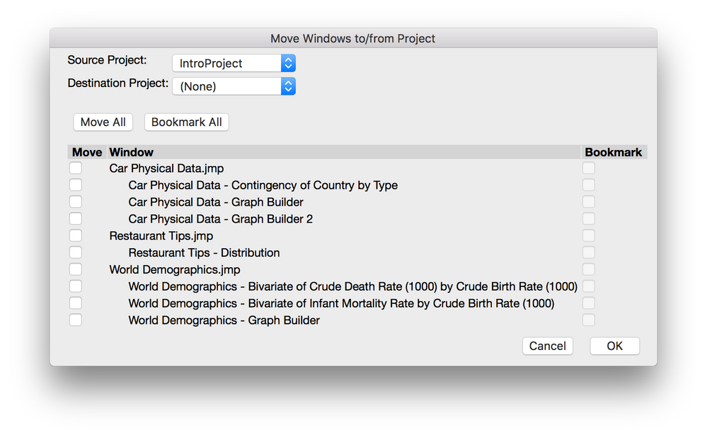
Many users will want to move from a project to multiple window mode, from multiple window mode to a project (using the project just for encapsulating a session), or from project to project (when a single analysis project gets to complex, for example). For that, use the Window > Move To/From Project as shown in Figure 3.
Simply pick the source project (or none if you want to move items from individual, separate windows) and destination project (which can be none, a new project or an existing open project). There are quick buttons for moving and bookmarking all files, or you can pick a subset of data tables and associated reports from source to destination.
Clicking a data table automatically brings over any report windows opened in the current project. If you don’t wish to keep them, simply close the tabs or windows after the move is complete. Data tables can also be bookmarked directly from this window. Also note that data tables must be saved on disk to be able to be bookmarked from this tool. Unsaved files can still be moved, however, to a new project or multiple windows.
Clicking on an individual line in the table brings up a useful thumbnail, which can help in deciding which files and associated graphs and reports are needed in the move.
Workspace Management
After files are added to the project, it’s time to configure graphs and reports into a tabbed arrangement using the workspace section of the project, as shown in Figure 1. By default, as new windows are created in a project, they are added in tabs that reside in a single column of the workspace.
Let’s look at a simple example project. First, create a new project and then immediately save it to the hard drive. Next, create a new folder called “sample project” and place the project file in that folder. By doing so, there is a single folder into which all of the scripts, data tables and supporting materials can be added. I’m going to create three groups in the project: Data Tables, Scripts and Output. Then I’ll add two files to the project: “FHPI.jmp” and “StatesMetadata.jmp.”
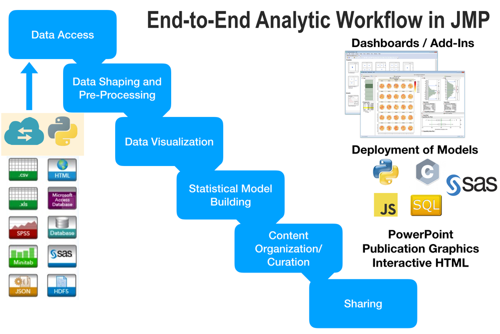
We’re going to use the project to write an automation script to develop a standard end-to-end analytic workflow consisting of data processing through a query script, data clean, visualization, modeling, content curation and final output for communicating results.
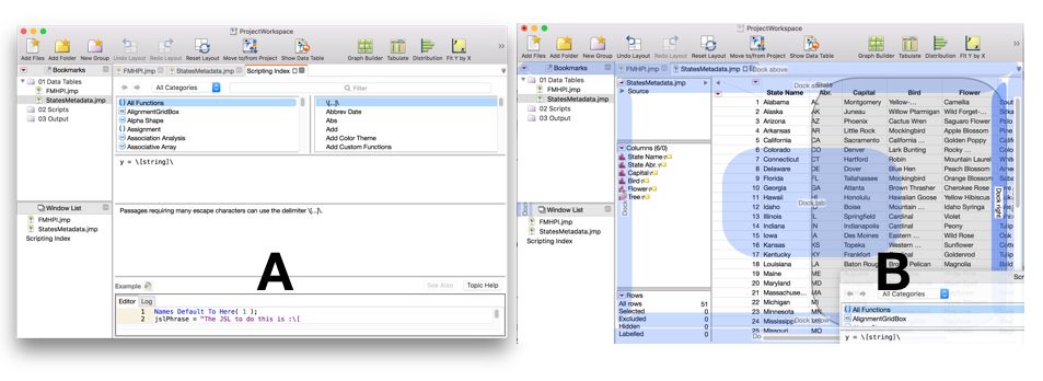
To begin developing the automation script, I can also instantiate that help > scripting index in case I need to look anything up. When the scripting index is loaded into the project, it is added as a tab. It would be more useful if I could dock it to the right of my data tables and output. To do this, simply peel off the scripting index tab. Graph Builder drop zones show up in the project, allowing you to drag and drop to reconfigure the project workspace, as shown in Figure 4.
Figure 4. Project workspace drop zones illuminated when a tab is peeled off a tab list. The drop zones are annotated for easier configuration of the project workspace.
Individual tabs can be maximized or minimized by clicking on the small tab icon on the tab title. This can be useful when, for example, you want to focus on an individual platform report or are using a platform, like Graph Builder, that benefits from a bit more real estate within the project. It can be also used for ad hoc presentations within the project.
When tabs are maximized, the Bookmarks and Window List remain. They can be hidden manually from the Project menu through toggling the Show Bookmarks and Show Window list commands. The project-wide log, which is hidden by default, can also be shown from this menu.
If at any point you rearrange the layout and don’t like the result, there is an undo and redo layout command to help. You can also go back to the default single-tabbed list by resetting the layout from the Project menu.
Tabs within the workspace can be navigated either by clicking on them (hovering over them with your mouse cursor produces a thumbnail), double-clicking within the window list or using the left and right arrows to scrub through the tabs.
Save and Archiving Projects
Continuing on with our analysis project, we are going to use the Query Builder to join our two tables together and create a third table, read for modeling and visualization. The Query Builder script can be built and then saved to the project folder. I’ll add it to the project and drag and drop it in the scripts group.
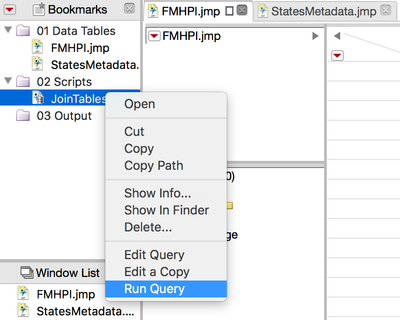
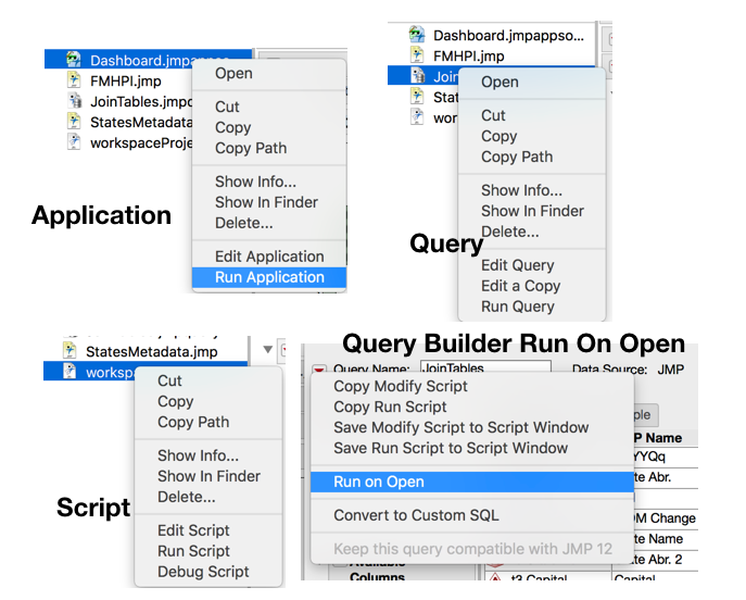
This is shown in Figure 5. Scripts, queries and applications or dashboards can be run directly through the right-click menu, saving you the click of opening it in the project and then running the script. It can also help keep the project clean, since there won’t be a tab open for a “production” script that is not being actively edited.
Figure 5. Running a script directly through right-click without opening it in a tab.
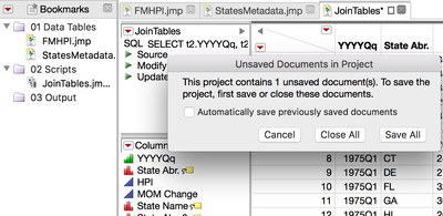
Running the script produces a third data table, with my two tables properly joined. The JoinTables tab has an * next to the name indicating that this file is not yet saved to disk. If I try to save the project from File > Save Project, I’ll get the following warning message, shown in Figure 6.
Figure 6. Unsaved documents in a Project warning message.
At this point, you have a decision about what you want to do, since all files must be saved or closed before a project can be saved. Clicking Save All will prompt you to save all the unsaved files to disk first and then will save the project. There is a checkbox, which is off by default, that lets you automatically save previously saved documents (with just unsaved changes) when saving the project. Use this setting carefully, especially when starting out using projects as you may make temporary changes to a data table that you wish to discard (adding columns, deleting columns, changing cells, etc.).
The Close All option will perform a close and no save to all unsaved documents but will keep you from having to save each document individually. This can be useful if you have a script that generates a lot of output, but you don’t necessarily want to save it.
You can also save unsaved documents manually, knowing that as soon as all of the * in the tab list are gone, you can save a project in a single click.
The project saves graphs and other platform output in a slightly different way. Since the project takes advantage of the session script functionality in JMP, graphs and platform output are automatically persisted upon saving and close without needing to save the scripts to the data table, to journals or saving the reports as .jrp files. This is especially useful to new users who want to save state of analysis projects without having to first learn any JSL.
Playing Scripts from Projects
Bookmarked .jsl, .jmpquery and .jmpapp/.jmpappsource files can be run from the bookmarks list directly (just like the Home Window in JMP). By right-clicking on any one of these files, you can see expanded options for what to do with these files, as shown in Figure 7.
Figure 7. Context menu for popular JMP file types in a project.
This right-click menu options allow you to quickly build an application, run a script or execute a query directly without having to open the AppBuilder/Dashboard Builder, Query Build or JSL script editor. The item will run and the results will automatically be opened in a new tab in the project, thus saving a click. Additionally, the Query Builder has an option to “Run On Open” (shown in Figure 7). This double-clicked query will be automatically executed without opening up the Query Builder.
Dashboards and Web Reports
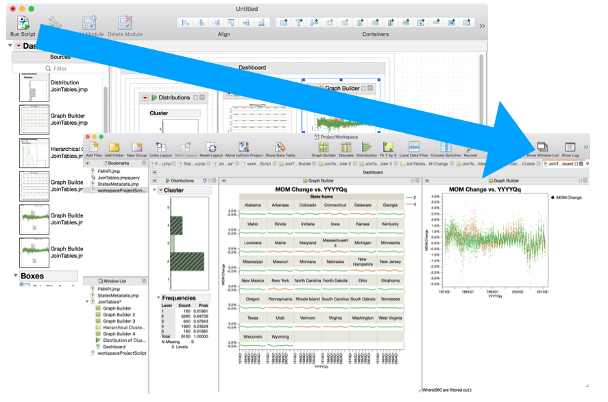
Dashboards and Web Reports are common ways to share and communicate results of a JMP analysis with others. Both features are supported with the JMP project. File > New Dashboard will open up the Dashboard Builder interface allowing you to see all of the available reports within the project. You can arrange the reports, add filters, text and other items; after clicking Run Dashboard from the red triangle menu, the resulting dashboard will show up in a new Tab in the project (see Figure 8).
Figure 8. Results of running a dashboard built with the Dashboard Builder within a project. The resulting dashboard will populate a new tab in the project.
Web reports are similar (File > Publish). The Create Web Report functionality will automatically see all available tabs within a project as applicable graphs to populate a web report. The web report can therefore be a good way to share the workflow of a project with someone who does not have JMP currently.
Case Study 1: DOE Project
Employing projects as part of design of experiments (DOE) within JMP can help in communicating results, as well as aiding in the work of the experiments themselves.
Using DOE in JMP means:
- Running the DOE platform to create the data collection scheme.
- Using the JMP table as a basis for data collection.
- Exploiting various JMP graphics platforms to view the results of the experiment’s runs.
- Utilizing JMP modeling platforms to build a predictive model based upon the data collected and as part of the modeling exercise, viewing various diagnostic plots to ensure a reasonable model has been developed.
- Constructing graphics and tables to communicate the results of the DOE with the intent of promoting action by an organization.
The generic procedure detailed above in Steps 1-5 often results in many windows and tables in JMP. It may also be true that the process can take months to move from Step 1 to Step 5, meaning that the JMP user has to save important results to her file system, remember where they are kept and keep track of the whole process.
This case study will use a simple experiment that anyone can run to show how projects can help with DOE by managing windows, tracking results and communicating conclusions.
I want to run a simple experiment to show how JMP Custom Designer can be used to perform experiments with constraints on a variable, such as total energy in this case.
The goal of this experiment is to find a good setting on my home microwave to cook popcorn. I have three variables in my control:
- Time (time in mm:ss that I can set for cook time).
- Power (an opaque Level 1-10, not sure what this means for temperature).
- Brand (there are many brands on the market; I’ve chosen the slightly disguised familiar brands Wilbur and Top Secret).
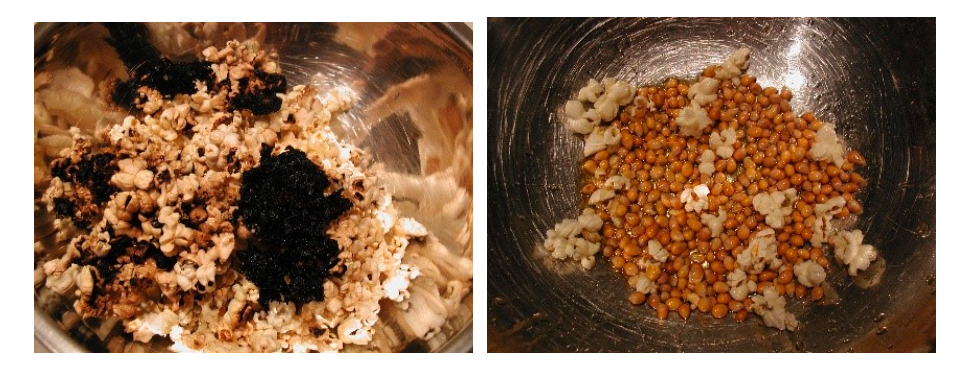
Per the instructions on the boxes of popcorn, I decided to vary the time from three to five minutes and the power from Level 5 to Level 10. I then set out to check the corners of the design space, meaning short time and low power and also long time and high power. These corners represent the maximum and minimum total energy of my chosen levels (Figure 9).
Figure 9: The left and right images above show the corners of the design space.
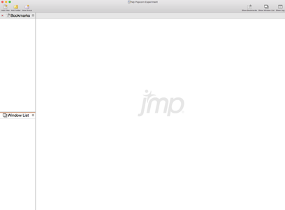
It is clear from my early results that the corners of the space are not feasible. So I will need to use the JMP Custom Designer to create a constrained design space. I want to use JMP Projects, so I first opened a new project and name it “My Popcorn Experiment” as shown in Figure 10.
Figure 10: Screenshot of an empty project at the start of the DOE workflow process.
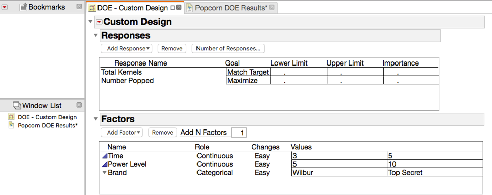
I then launched the Custom Designer within the project and set up my responses and factors as shown in Figure 11.
Figure 11: Launching Custom Desig to set up the experimental runs.
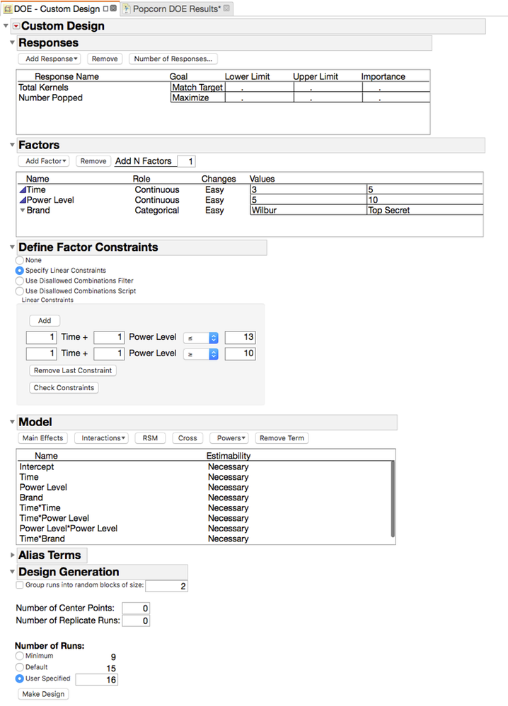
Now it is time to choose my model (RSM) and set the constraints on total energy (Time + Power Level). Setting linear constraints on the factors is done by simply setting up the constraints as shown in Figure 12.
Figure 12: Setting up the experimental constraints and adding the effects that I want to be able to model to determine the number of runs needed.
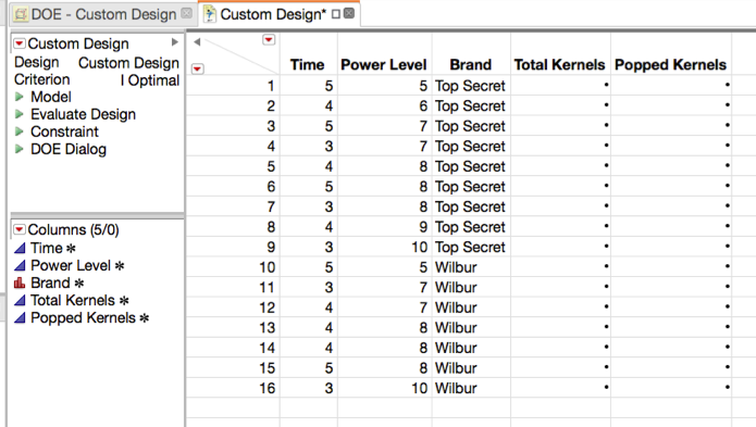
I chose Make Design, resulting with JMP showing a candidate design. Figure 13 shows the design I used with formats of time and power level that match what I can set on my microwave.
Figure 13: Experimental run table.
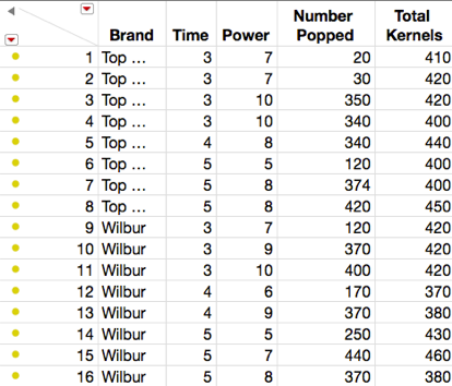
Next, I popped 16 boxes of popcorn. Using a cup measure as a sampling tool, I selected a representative cup from each run and counted the total kernels and number of popped kernels. The data are as seen in Figure 14.
Figure 14: Results of the experiment.
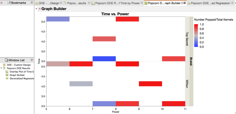
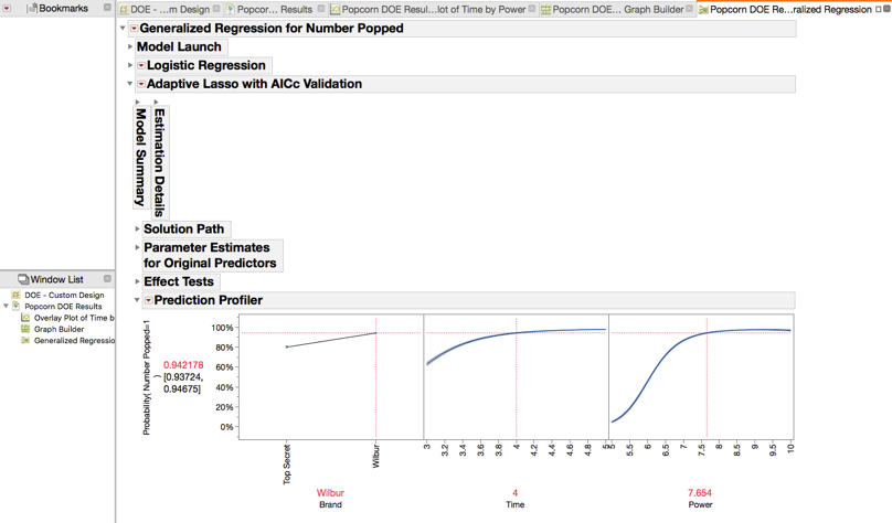
I looked at a few graphs and built a generalized regression with the Number Popped as a binomial response. A heatmap of Time vs. Power by Brand with the ratio of Popped to total colored from low (blue) to high (red) shows that mid to high combinations of Power Level and Time have better results. A profiler of the regression model best communicates the results with the added conclusion that Wilbur branded popcorn is more robust to total energy. Figures 15 and 16 show these results.
Figure 15. A heatmap of Time vs. Power by Brand with the ratio of Popped to total colored from low (blue) to high (red).
Figure 16: Profiler showing the final model and the effects of changing brand, time and power factors on the response.
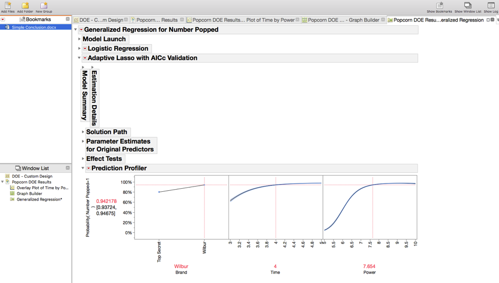
Finally I wrote a Simple Conclusion document adding two graphics as PDFs from JMP; I added this conclusion document to the project by selecting the Add Files button on the upper left of my project window as shown in Figure 17.
Figure 17. Bookmarked simple conclusion for sharing the results of this experiment.
I now have a project file that contains my design setup, data, model and supporting graphics, as well as conclusion document. This is a self-contained file that is the basis of my memory of this experiment. It also serves as a corporate memory of this experiment if I store the project and supporting files in a location that can be retrieved by members of my team now and in the future.
Case Study 2: Predictive Modeling Project
We are going to use to project to assist with the task of building a model to predict wine quality from a set of physicochemical properties (see Cortez et al. 2009). The data set is available to download from the UCI Machine Learning Repository (Lichman 2013). We can use the project to manage the process of importing the data via Multiple File Import, exploring and cleaning the resulting imported data table, building graphs, building a number of candidate models using various machine learning techniques in JMP Pro, comparing models, deciding on a model to use and ultimately generating score code to aid in putting this modeling into production. We’ll be following the end-to-end analytic workflow in JMP (See Figure 18) to demonstrate how the project naturally supports the process.
Figure 18. End-to-end analytic workflow in JMP.
The historical data is available for download from the UCI Machine Learning web site directly: http://archive.ics.uci.edu/ml/datasets/Wine+Quality. There are three files to download: winequality-red.csv, winequality-white.csv and winequality.names. The first step in creating a project is to go to File > New Project in JMP as well as make a folder on the desktop called “Wine Modeling Project.” I’ll place all three of the text files into this folder.
I’ll save the project file into the wine quality project folder and then create several groups to help me organize my bookmarks: 01-Raw Data, 02-JMP Data Tables, 03-Scripts, 04-Score Code, 05-Output.
I’ll bookmark all three of the raw data files by dragging and dropping them from the finder to the raw data folder.
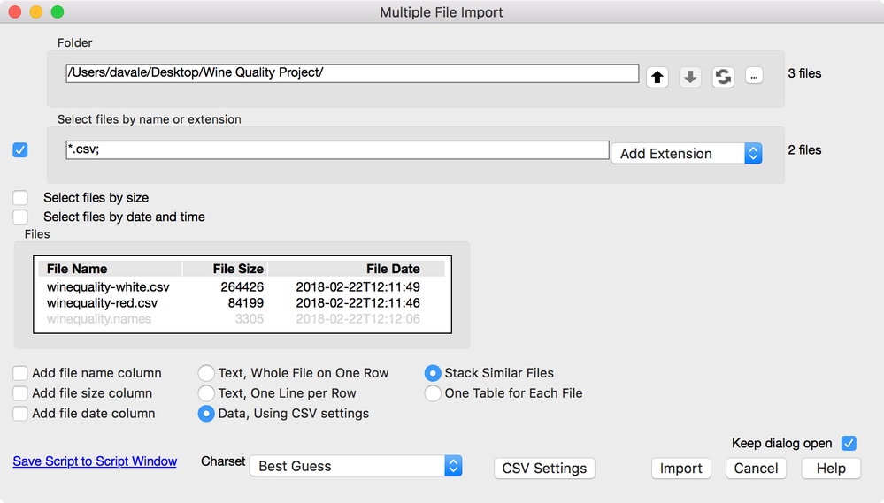
Next, I want to get the files into a JMP data table. I’m going to use the Multiple File Import to automatically open both CSV files and concatenate them without needing to write a script or use the tables menu (File -> Open Multiple…). To just open the .csv files, I’ll make sure to select by extension: .csv. and keep the radio button checked for stack similar files. I’ll check the Add File Name Column so that I’ll maintain which samples are red wine and those that are white. I’ll save script to the script window and save the script to the project, so that if new data comes in and I want to regenerate the JMP data table, I can do it directly without having to go through the dialog again of the Multiple File Import (Figure 19). I’ll bookmark the script for later by dragging it from the window list to the bookmarks and then close the script.
Figure 19. Multiple File Import settings.
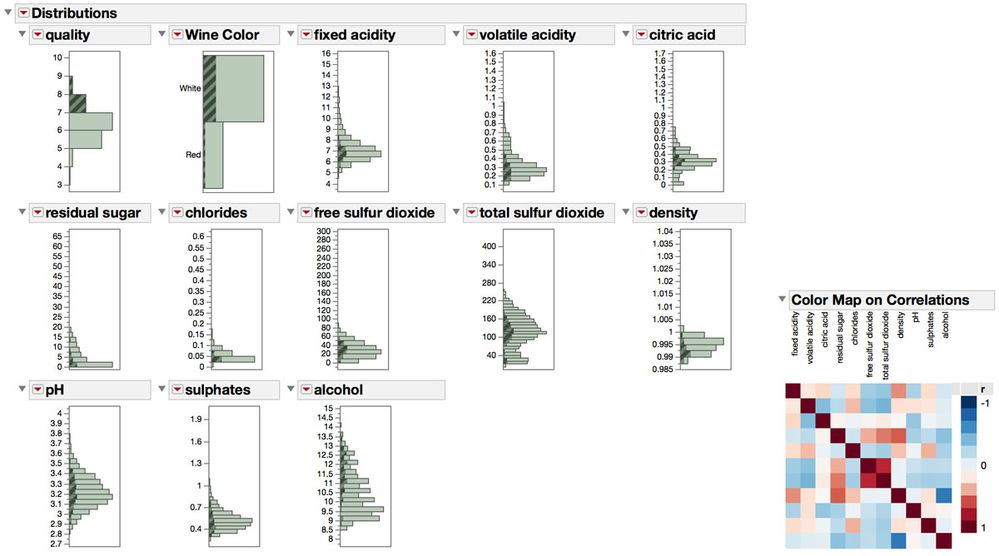
Now that my data sets are open into a single JMP data table, I’ll save the file and then bookmark it in the project. I can use Recode to add a column (Color) which shows the category of the wine in that sample. The goal of this modeling exercise is to use the relatively inexpensive method of measuring physicochemical properties (like residual sugar, alcohol, or sulfites) to predictive the relatively expensive to gather professional taste tests of the wine. We are fortunate to have the historical data, which has both properties, and we can use good cross-validation techniques to build a model on this historical data, which may work well on new data where we only have the physicochemical properties available to us. Figure 20 shows a distribution matrix with high-quality wines selected. We can see in the distribution of the other measures that there may be some separation in some of the values to segment these highly rated wines (i.e., higher-quality score wines appear as if they tend to have lower residual sugar and higher alcohol content). We will test this hypothesis by building several models.
By performing a multivariate analysis and looking at the Colormap on Correlations, we can also see that many of the measures are highly correlated with each other, which will prove challenging for standard modeling techniques like stepwise regression or least squares.
Figure 20. Distribution matrix of physicochemical properties, color and quality scores. Highly rated wines are selected. Color Map on Correlations for the physicochemical properties are shown on the right.
In order to assess the model performance and give our various modeling techniques the same shot at predicting wine quality, we are going employ cross validation for honest assessment of model performance. Basically we are going to separate the data that we have into three sets: training (used to build the models), validation (used to fine-tune the models and balance complexity and parsimony with performance) and, finally, test (a subset of the data not used in modeling, but only used to simulate new data coming in and therefore our judge of the model’s ability to perform on new data).
To build the validation column, I’ll use the Make Validation Column utility in Analyze > Predictive Modeling. I’ll choose the option for stratified random and then click on the Wine Color column to assure that I have equal proportions of samples in train, validation and test groups for both red and white wines. I’m going to do a 70%/20%/10% sample of train, validation and test groups.
We are going to build several candidate models and then publish them to the Formula Depot. The Formula Depot fits nicely in a project. I’ll bring it up (Analyze > Predictive Modeling) and then dock the Formula Depot in its own column to the right of the project.
Now we will build a Boosted Tree, Bootstrap Forest, Neural Net and Several Generalized Regression Models. As I build the individual models, I’ll publish the results to the Formula Depot.
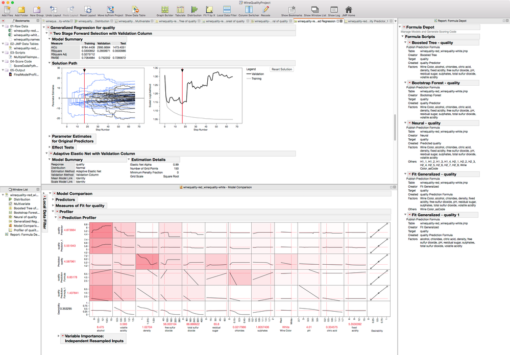
Figure 21. Final predictive modeling project.
It appears as though the Bootstrap Forest is the model that provides the best fit to the test data. The Bootstrap Forest has captured the underlying model form well. Figure 21 shows how I might setup the project to see all the models I’ve built in a tab list with the collection of models in a Formula Depot docked to the right of the workspace and a model comparison directly underneath the model output to look at variable importance and a profiler for the various candidate models.
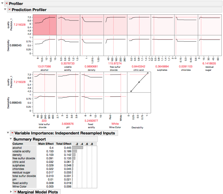
What the Bootstrap Forest does well is capture the fact that increasing the alcohol of the wine increases the quality to a point, as shown in Figure 22. This figure shows the settings required to produce the highest quality wine as indicated in the historical data. We can share these results with others in two ways. One, by saving the model’s score code from the Formula Depot in a variety of languages (like SAS, Python, C, JavaScript or SQL), and also to PPT or HTML.
Figure 22. Bootstrap Forest model predicting wine quality.
This interactive report can be shared with others that don’t have JMP. And the Profiler remains interactive on the Web so the values can be adjusted interactively to see the impact on Wine Quality. Both the model score code and interactive HTML5 report can be bookmarked in the project as well.
References
- Cortez, A. Cerdeira, F. Almeida, T. Matos and J. Reis. Modeling wine preferences by data mining from physicochemical properties.
In Decision Support Systems, Elsevier, 47(4):547-553, 2009. - Lichman, M. (2013). UCI Machine Learning Repository [http://archive.ics.uci.edu/ml]. Irvine, CA: University of California, School of Information and Computer Science.
