- JMP User Community
- :
- JMP Discovery Summit Series
- :
- Past Discovery Summits
- :
- Discovery Summit 2018 Presentations
- :
- A Good Query Can Set You Up for Success ( US 2018 117 )
- Subscribe to RSS Feed
- Mark as New
- Mark as Read
- Bookmark
- Subscribe
- Printer Friendly Page
- Report Inappropriate Content
A Good Query Can Set You Up for Success
Level: Beginner
Brian Corcoran, JMP Director of Research and Development, SAS
JMP provides a variety of ways to get a wide range of data formats into the product. The reason is obvious enough. There are a lot of tools that were developed over the years to collect and format data. In most cases these tools don’t allow you to convert your data to JMP Data Tables. You need to get this data into JMP for analysis. In other cases, the data may be in a database somewhere, and you need to extract it before starting. Getting the data in can consume valuable time. JMP has evolved over the years to add powerful data acquisition capabilities to aid you in this task.
This paper attempts to give a small sampling of how to use the Query Builder capabilities in JMP, along with a simple example of using the Excel Wizard. Hopefully it also shows that the journey can also be the reward, in that insights into the data can be gained from preparing the query itself. While the Windows version is used for the desktop screenshots, all the facilities discussed here are also available in the Mac version of JMP. JMP 14 was used, but JMP 13 can do everything discussed as well.
This paper presents a hypothetical usage case. Imagine that you are studying world trends and that the World Bank database often provides valuable information. A colleague tells you that the 2017 World Development Indicator data has recently become available, and that they have put the data into the company SQL Server database. This is a large table, with over 400,000 observations and 62 columns. [1] You open JMP up and select File->Database->Query Builder, open your database connection and point to the table. In first screen of Query Builder, you select the world_bank table as your primary table and use “Table Snapshot” to take a look:
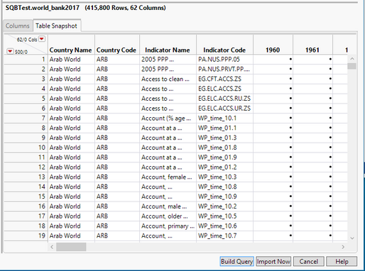
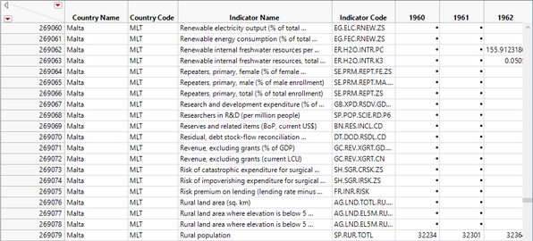
It is somewhat of a strange format, at least for a typical JMP user. There are four variables or columns for country information, and then a column for every year data is present. The rows have what appears to be a region and then the data being measured. In some respects, it looks the opposite of expectations for a typical JMP table. The Country Name “Arab World” appears to represent a region, so this also is confusing. If you press the “Import Now” button the table comes in and things become a bit clearer. By scrolling to the middle you can see that rows start with the country in question, and then the bit of data for a particular subject, like “Rural Population”. This is all sorted by country, which doesn’t seem intuitive.
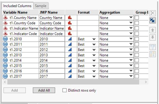
Let’s start over. This time, we can go ahead and select “Build Query” rather than “Import Now”. We know we want the first four variables with country information, so we can select those and press “Add” in the Included Columns tab of the column selection panel in Query Builder. There is a lot of data here, so let’s just do the variables for 2010-2017. At this point, the top of the dialog looks like:
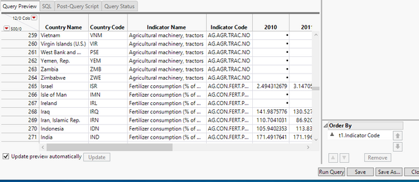
There are still problems with the data. First, it has regional groupings that are not of interest right now. How to exclude these aggregate entries? Also, what would be the best way to query a specific item, like “Fertilizer Consumption”?
It certainly would be possible to import all of the data into JMP and then delete the regional groupings if we don’t Order By “Indicator Code”. However, that puts a burden on the person analyzing the data. If that is somebody not setting up the query, that could be confusing. Within the query, it would be possible to just select the countries that are of interest. What if we want all the countries in the European Union? (I was going to use North America, but the World Bank definition only contains the U.S., Bermuda and Canada!) We could manually select them, but there is a better way. To do that, we are going to quickly invoke another tool in JMP, the Excel Wizard.
In this scenario, suppose that we operate on data from the World Bank often. The country codes are important, but not intuitive. Tables often use the codes without specifying the full country name, as you can see from looking through the website. It might be handy to have those codes in a separate table. Such a table exists and is easily imported from the website as an Excel file. So, in this case open up the Excel Wizard on the table of countries and country codes. The World Bank website groups these in an obscure table called CLASS.xls, but you can rename it. There are two tables within the file, “List of economies” and “Groups”. Let’s look at “Groups”:
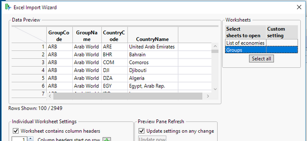
There is the grouping for Arab World that we saw in the Query Builder data. This looks promising, but scrolling down doesn’t show Europe yet as the preview ends at 100 rows. Select “Show all rows” and we can see everything, including “Europe & Central Asia”, “Europe area” and “European Union”. The “European Union” group contains the country codes for all the countries currently in the union. Could we use this to select the countries within Query Builder? The answer is yes, so let’s go ahead and extract just that group that we need. We can do that by selecting the first row in the preview with “European Union” and then pressing the green plus next to “Data starts on row”.
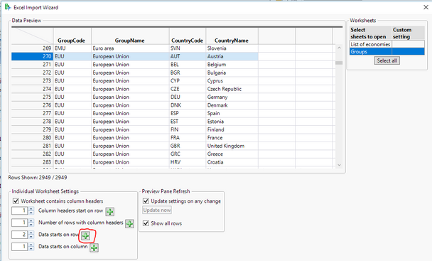
Now we can press the “Next” button on the dialog, select the last row with “European Union” and press the green plus next to “Data ends with row”. This reduces the data to just the countries that we are interested in.
Now we can select “Import” and get a row with 28 entries for the countries in the European Union. We’ll go ahead and save that resulting JMP table as “EU.jmp”.
Now we can return to Query Builder. We could have selected the countries that we are interested in with a tedious process of selecting them in a list by “Country Name” or “Country Code”. However, Query Builder has a powerful filter type called Match Column Values. To use this, we first drag “Country Code” into the Filters pane. This will produce a long list with every code in it. Now, we can select the red triangle menu at “t1.Country Code” for Filter Type and select “Match Column Values”. A box showing the names of open JMP tables will be presented. Since we still have “EU.jmp” open, it shows up in the list. We select it, and the variable (CountryCode) that we want to match. It is also important to make sure that “All Rows” is selected from the dropdown list, rather than “Selected Rows”, since we want all the countries in this case.
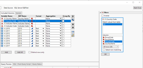
This will reduce our results to only the observations where an EU country is involved. There’s really no magic here. We are building a WHERE/IN clause to substitute the country codes. If you look at the SQL pane within the Query Builder you can see the SQL that JMP is generating:
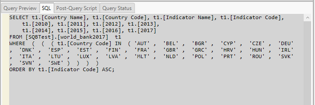
But hopefully we’ve made the process a lot easier to accomplish. Now that we’ve narrowed down the data to what were are really interested in, it would be nice to make it easier to select the specific information that we would like to analyze. To do this, we can drag “Indicator Name” over to the Filters pane. While we could click on the item we are interested in here, and then run the query, it would be nice to be able to have a more interactive interface for any user. We can press the red triangle menu by “t1.Indicator Name” and select “Prompt on Run”. This will present us with a dialog to specify the title for the prompt to the end-user.
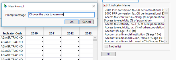
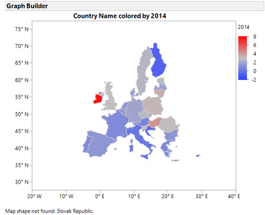
Now, when we press the “Run Query” button, we will get the list of items and we can select the one that we are interested in. For example, we can select “GDP Growth (Annual %)” and get a 28 row table. We can then put that into Graph Builder. Dragging the “Country Name” into Map Shape drop area will produce a map of Europe, and then we can drag the year of interest in. Data starts to get sparse after 2014, so doing that year produces:
JMP is looking for “Slovakia” rather than “Slovak Republic”, so that may be an opportunity to use Recode. In looking at this data, it seems like we will always be doing a similar operation. We will select the Country Name for the Map Shape, and then the year that we are interested in to examine the results. If we are going to be looking at a certain year repeatedly, it makes sense to save the script and put it into Query Builder as a Post-Query Script. There is a tab by the preview pane for this. If we go to our previous graph and, using the red triangle menu do Save Script->To Script Window we will get a script that looks like this:
Graph Builder(
	Size( 534, 454 ),
	Show Control Panel( 0 ),
	Variables( Color( :Name( "2014" ) ), Shape( :Country Name ) ),
	Elements( Map Shapes( Legend( 7 ) ) )
);
If we paste this into the Post-Query Script tab, when we select the observation that we want to examine, it will always run the same Graph Builder report after the data is extracted and the JMP table is created. This can greatly simplify a repetitive task.

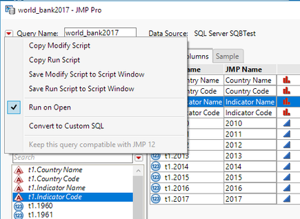
The best part is that when we save the query, we can set it so that an end-user doesn’t even see the Query Builder dialogs. By selecting “Run on Open” in the drop down menu by the Query Name field, and then saving the query, the end-user will only see the prompt and the resulting table and graph.
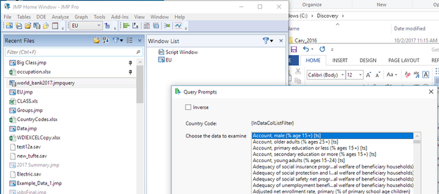
At this point, we have filtered through a large amount of confusing data and created a repeatable query and analysis that we can ship to an end-user. The person using the query would not really need knowledge of the query, or really of much of JMP at all.
Conventions used:
Query Builder window panes are bolded
Buttons / Dialog controls are “quoted and bolded”
Variables / Column names are “quoted and italicized”
[1] World Bank Group. World Development Indicators, World Bank Group, n.d. Web. January 25, 2018. https://datacatalog.worldbank.org/dataset/world-development-indicators . Obtained under Create Commons CC BY 4.0 license.
- © 2025 JMP Statistical Discovery LLC. All Rights Reserved.
- Terms of Use
- Privacy Statement
- Contact Us
