Solving Common Data Table Problems With JMP® 13: Can We Replace Summary and Join With the New JMP Query Builder?
Daniel Valente, PhD, JMP Senior Product Manager, SAS
Jon Weisz, JMP Vice President of Sales and Marketing, SAS
Abstract
JMP 13 introduces two new tools that make it easy for the analyst to deal with common data problems. Often two or more data tables are related by a common key, yet they are very different in terms of fact-sampling frequency or dimensions (e.g., long versus wide). Doing an actual join of these two (or more) tables may create a resulting table that becomes very large in memory. While this is a nuisance when the fact and dimension tables are relatively compact, it can quickly generate a joined table that is too big to fit in memory. The solution is to use a virtual join, which preserves the joined relationship without actually creating the joined table – effectively enriching the fact table without burdening it. Analysts often find themselves needing to make complex table joins or summarizations in database and writing SQL, which create their own set of pains, particularly when there are complex relationships like slowly changing dimensions. JMP Query Builder serves as an easy SQL-generating and writing tool, whose code can then be executed in a database. After you drag and drop the correct and desirable query, Query Builder automatically writes the SQL code for you, obviating the need for tedious manual and error-prone work.
Overview of Relational Table Structures
Analysts need data in a form that has variables in columns and observations in rows. The data may also need categorical columns that clearly subgroup the observations (e.g., income level, country, machine, etc.). The data also may have attributes that further illuminate observations (e.g., address, serial number, customer ID, etc.).
Often the source data for such analysis are relational data structures stored in databases. Many modern courses of study in data science cover topics related to relational data structures, databases and SQL. But most engineers, scientists and statisticians are not exposed to these topics in an academic setting, so they must learn about them as part of ongoing, informal education. JMP Query Builder offers analysts a bridge between relational data structures and analysis-ready data. By learning a few terms and concepts, analysts can use Query Builder to generate data that is ready for analysis.
The brief discussion of relational data structures in this paper is not meant to replace a thorough study of the topic; rather it introduces the terms and definitions used when working with Query Builder and its virtual join capabilities in JMP.
Why have more than one table to store important data?
Imagine you need to devise a way to store data about customers’ purchases of your company’s products. You might first start by listing all the variables that may need to be collected, such as:
- Purchase Date
- Purchase Amount
- Purchase Method (PO or CC)
- Product SKU
- Product Description
- Customer Name
- Customer Address
- Customer Phone Number
This is certainly not a comprehensive list, but it is a good start. Now think about maintaining these data. This table will have eight columns and one row for each purchase. Some fields may have many distinct values, like Purchase Amount or Purchase Date. Other fields will have far fewer distinct values and many repeated values, like Product SKU and Description.
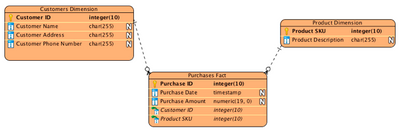
A common way to reduce the size of the table is to break the table into three logical groups. First is the table containing transactions or facts, such as Purchase Date and Purchase Amount. The second table would have the customer information, and the third would have the product information. To maintain the links between the data columns, a column with link information would have to be added to relate the three tables. These columns are called keys. A common way to show this layout is to employ an entity relationship diagram (ER). Each entity has a table name, a key or set of keys that uniquely identify each row, and a set of attributes or variables the give information about each row. The ER diagram for the customer purchase date is shown in Figure 1.
Figure 1. Entity relationship diagram for customer purchase data
The key symbol next to Customer ID in the Customers Dimension table means that if you know a Customer ID, you can uniquely find that customer in the table and all associated information. The Customer ID is also in the Purchases Fact table. The Customer ID is called a Foreign Key when it is in the Purchases Fact table because it may appear many times and uniquely defines rows in a foreign table to the one it appears.
With the layout in Figure 1, it is very easy to see how to update a product description. To do this, you would just have to edit the Product Dimension table and that one change would apply to all purchases ever made, a benefit referred to as maintainability. If this was one table with the Product Description repeated many times, you would have to edit many rows, which would inevitably lead to mistakes and data quality issues.
Case 1: Current Population Survey
Now let’s look at an example with Query Builder. The US government collects a lot of interesting data with the Current Population Survey (CPS)[USGCPS]. The CPS is:
“The Current Population Survey (CPS) is one of the oldest, largest, and most well-recognized surveys in the United States. It is immensely important, providing information on many of the things that define us as individuals and as a society – our work, our earnings, and our education. In addition to being the primary source of monthly labor force statistics, the CPS is used to collect data for a variety of other studies that keep the nation informed of the economic and social well-being of its people. This is done by adding a set of supplemental questions to the monthly basic CPS questions. Supplemental inquiries vary month to month and cover a wide variety of topics such as child support, volunteerism, health insurance coverage, and school enrollment. Supplements are usually conducted annually or biannually, but the frequency and recurrence of a supplement depend completely on what best meets the needs of the supplement’s sponsor.”
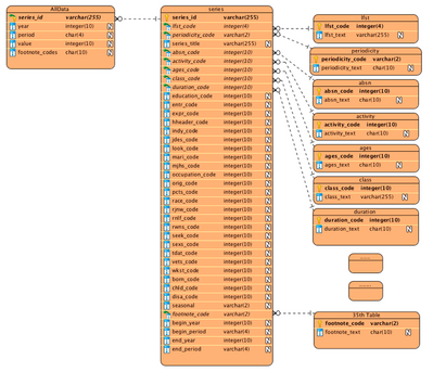
These data are available to download as 36 text files, which are easily opened in JMP since the files are tab delimited text files. Looking at the JMP tables, an ER diagram (Figure 2) was created to inform the work in Query Builder.
Figure 2. ER diagram for the CPS labor force statistics data tables
To use Query Builder, you will need to define a Primary Table (fact) and Secondary Table(s) (dimension).
The fact table for the CPS data is called AllData.jmp. The table has more than 5 million rows but only five columns. The columns have a “series_id”, dates and a “value” column. To make any sense of the data, you need to find out what the series_id.jmp means. The ER diagram in Figure 2 shows that “series_id” is related to the series.jmp table. Next, open both those tables in JMP and use Query Builder define the join.
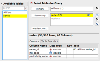
In JMP, select AllData.jmp as the Primary (fact) table and series.jmp as the Secondary (dimension) table (Figure 3). JMP will automatically look for keys that fit and set up the join, but you should verify it by clicking on the Venn diagram to the right of the series table. Query Builder found “footnote_codes” in both tables, but you do not want to join on those as key, just the “series_id,” so that key relationship should be removed.
Figure 3. Query Builder for the join of AllData.jmp and Series.jmp
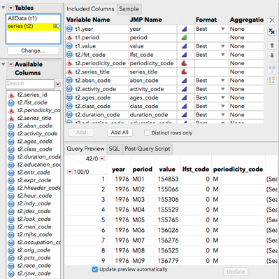
Now you need to define the columns in the joined table (Figure 4). To do that, select AllData.jmp in the upper left and select the columns needed from that table. Drop “series_id” now, because you will not need that key in the resultant table (series and data.jmp).
Figure 4. Query Builder to join series and data.jmp to all “_code.jmp” tables
Notice that series and data.jmp is about five times larger than the AllData.jmp table. This inflation is due to the repeated values of all the “_code” fields. So clearly the storing of the data in 36 tables reduces the storage requirements substantially. Next, select series and data.jmp as the primary table and all the “_code.jmp” tables as secondary tables (Figure 5).
Figure 5. Query Builder to join all the “_code.jmp”
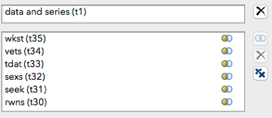
Build the query with only the “_text” fields from the “_code” tables because you no longer need the key variables. Using the Cols > Columns Viewer in JMP, you can easily get a summary of the now 42 columns in the table Full join.jmp. You will still have 5.7 million rows, which is the same as AllData.jmp, but now you have the text fields that describe the data. Even though the table Full join.jmp is still six times larger than the table AllData.jmp, you now have a table useful for analysis.
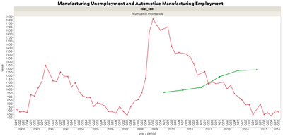
Use Graph Builder to plot manufacturing unemployment trend from Full join.jmp. In Figure 6, the disruption in this sector during the recession is shown with the red trend line. Unemployment levels in 2016 are back to the levels seen in 2006-2007. The green trend line shows employment levels for the automotive manufacturing sector. More than 300,000 automotive manufacturing jobs were added from 2010 to 2015.
Figure 6. Graph Builder showing data from CPS labor force statistics
Case 2: Restaurant Inspection Data
This case explores using virtual join and JMP Query Builder for analyzing the DOHMH New York City Restaurant Inspection Results [DOHMH]. Imagine yourself as a new inspector on the job and exploring some historical data to see what the data reveal. From the website https://data.cityofnewyork.us/Health/DOHMH-New-York-City-Restaurant-Inspection-Results/xx67-kt59, you can download a .csv version of these data that can be easily opened in JMP. The full download on July 17, 2016, generates a 163.3 MB file that includes 448,149 records.
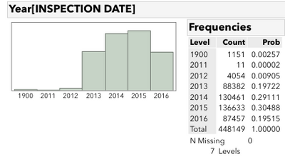
These data have an INSPECTION DATE column, which is a M/D/Y of the inspection event. To see how many years are included in these data, right-click and use a New Formula Column > Date Time > Year. Converting that from continuous to nominal and then Analyze > Distribution is shown in Figure 7. The level 1900 is likely a code for missing data, something that you will need address. It’s not a problem to destructively edit these data (since JMP is used as a sandbox here and the real data is always stored on the server); next use the Recode utility to change these levels to missing.
Figure 7. Inspection Dates for full data set
In the recode window, there are 1,151 records that are 01/01/1900. Change this old value to • by deleting the string and then clicking Done -> In Place. Since the RECORD DATE is the date that the data was pulled and not material to this analysis, delete the column.
This paper is about virtual join and Query Builder, so you might wonder why we are looking at a denormalized table. There seems to be an opportunity to normalize these data. Notably absent from these raw data is the geocoded location of the individual restaurants, a task that can be performed with with a JMP Add-In later. Since this process is expensive computationally, it makes sense to only geocode unique locations, which may have multiple inspections in these data. Additionally, there seems to be an opportunity to have an additional table of violations, which are far fewer than unique inspections.
Before splitting the data, take a sample of these data so that the numbers will be more manageable for your exploration exercise.
Sampling is something that can be performed easily with Query Builder. Tables > JMP Query Builder will bring up the launch dialog. Because you are not performing a join in this case, use DOHMH_New_York_City_Restaurant_Inspection_Results.jmp as the Primary Table with no Secondary Tables at this point. In Query Builder, there is a tab named Sample. Turning on the check box for “Sample this results set,” you can choose First N rows or Random N rows. Take a random 10 percent sample of these data, so put 44,815 in the Random N rows. Add all the columns to the Include Columns section and then inspect the SQL. Query Builder has automatically generated the SQL to perform this query:
SELECT t1.CAMIS, t1.DBA, t1.BORO, t1.BUILDING,
t1.STREET, t1.ZIPCODE, t1.PHONE, t1."CUISINE DESCRIPTION",
t1."INSPECTION DATE", t1."ACTION", t1."VIOLATION CODE", t1."VIOLATION DESCRIPTION",
t1."CRITICAL FLAG", t1.SCORE, t1.GRADE, t1."GRADE DATE",
t1."INSPECTION TYPE", t1."Year[INSPECTION DATE]"
FROM DOHMH_New_York_City_Restaurant_Inspection_Results t1
ORDER BY RANDOM() LIMIT 44815;
After using the Order By Random () function for our sampling, this query will generate the appropriate subset of the data. Save this as a subset and then split off the restaurant demographics and violation codes. Query Builder can also be used here. Start with the violation codes. Again, you just need a Primary Table. Drag and drop VIOLATION CODE and VIOLATION DESCRIPTION to the variables listing and then drag in the VIOLATION CODE again, which lets you aggregate by count and generate the table that has the desired properties. Change the JMP Name of the aggregation column to VIOLATION COUNT. This ability to generate an alias to a column or derived column is a powerful feature of Query Builder. You can also choose to automatically sort by the newly created aggregated column by dragging the VIOLATION COUNT to the Order By role, shown in Figure 8.
Figure 8. Aggregation column renamed as Violation Count, with an Order By property
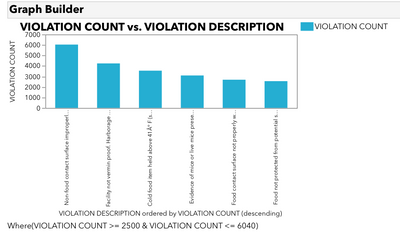
With only 88 unique Violation Code, this resulting query is much more compact. After naming this table D-ViolationCodes.jmp, this is a good time to use Graph Builder to explore which codes have the most records. Drag VIOLATION DESCRIPTION to the X axis and VIOLATION COUNT to the Y axis. Then right click the VIOLATION DESCRIPTION and Order By VIOLATION COUNT (descending). To focus on just the top categories, you can use the Local Data filter on VIOLATION COUNT with violation categories, which have more than 2,500 unique records (Figure 9).
Figure 9. Top violation counts (>2500 unique records in the sampled table)
Moving away from the violation table for now, you can focus on the unique restaurant demographics. At this point, you can also delete the violation description, which saves a number of duplicate rows in the main fact table. Use the VIOLATION CODE, which is a much more compact way to organize these data (three-letter strings vs. sentence-long strings).
Again, use Query Builder to peel off the unique restaurant demographics. It’s very likely that there is more than one pizza shop of the same name in NYC, but Query Builder can handle that situation. The column CAMIS functions as an ID that can be used to identify unique restaurants. In Query Builder, drag in CAMIS twice, one of which should be Aggregated by count and renamed INSPECTION COUNT. The rest of the demographic data is DBA, BORO, BUILDING, STREET, ZIPCODE, PHONE and CUISINE DESCRIPTION. Finally, calculate a column called ADDRESS for the geocoder, which will be done as a post-query script. Run the Query and then utilize a formula column with the following formula:
:BUILDING || " " || :STREET || " " || :BORO || " NY," || Char( :ZIPCODE )
This formula puts together the correct address. Typing :ADDRESS << get script; in a script editor will produce the JSL required to generate the column for a post-query script. Copy and paste that code into the appropriate tab in Query Builder and then generate a column that will split the data into 20 groups for a better interface with the geocode. After generating a new column called Group and Initialize Data: Sequence Data, From 1 to 20, Step 1, Repeat 1, you can get the script and paste it into the post-query script. Now that both columns are scripts, you can delete the query table and rerun the query. Save this data table as D-Restaurants.jmp. As a final step, delete the extra columns from the now fact table including: DBA, BORO, BUILDING, STREET, ZIPCODE, PHONE and CUISINE DESCRIPTION.
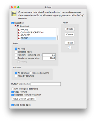
Save this table as F-Inspections.jmp. Now you are ready to geocode the groups of restaurants with an add-in created by Xan Gregg available on the JMP File Exchange [GREGG], which uses OpenStreetMaps.org to geocode locations. This service is expensive computationally and prone to failure so it’s best to split up D-Restaurants by group using Tables > Subset. The Subset By functionality of this platform, shown in Figure 10, is useful here.
Figure 10. Subset tables platform for splitting by restaurant group
The newly created 20 tables can be individually geocoded using the add-in. The address field helps determine the correct latitude and longitude. And finally, save the results to the same data table.
To get the data table back to a single dimension table with locations, use the Tables > Concatenate function, combining the 20 groups; it is named D-RestaurantswLocation.jmp.
Now that you’ve broken down this table using Query Builder, you can build it back up using virtual join.
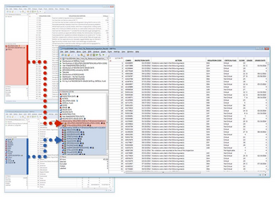
First, start with our two dimensions tables: Restaurants-wLocation.jmp and ViolationCodes.jmp. Right clicking on the VIOLATION CODE and selecting Link ID will set up the start of the virtual join. Notice a small key icon shows up in the columns list. Move to the Restaurants table and do the same with the CAMIS. To finish up the virtual join, move to the fact table, which has all the inspections and then select Link Reference for both the CAMIS and VIOLATION CODE.
All the columns show up in the fact table without having to physically join the tables in memory. The virtual join can also be scripted through a column property:
For the Link Reference:
Set Property("Link Reference", Reference Table("D(f)-Restaurants-wLocation.jmp"));
For the Link ID:
Set Property("Link ID", 1);
Figure 11. Virtual join
Figure 11 shows that you have access to the columns in both of the dimension tables without burdening the fact table.
Finally, build a dashboard to visualize and explore these data leveraging the virtually joined columns.
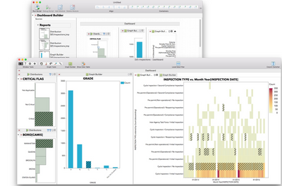
Figure 12 shows how Dashboard Builder displays a collection of five graphs. To use two of the graphs as selection filters, start with the Hierarchical Filter template in Dashboard Builder, using the CRITICAL FLAG and BORO as the Filter and Hierarchical Filter. Next, use a graph of the grade counts, the mean score by quantile on a map and, finally, a heat map of the date counts by type of inspection.
Figure 12. Dashboard Builder mode of Application Builder with Final NYC Inspection Dashboard
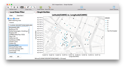
This is just an example of the type of visualization you can make with these data, leveraging the linked tables afforded by the virtual join. The geocoded data also allows, for example, you to dig into the locations of restaurants by cuisine (Figure 13).
Figure 13. Geocoded restaurants colored by grade showing on a street level map
SQL Generation and Deployment
Another major advantage of using Query Builder is the generation of Structured Query Language (SQL). SAS can use SQL within Proc SQL, and most databases use SQL as a programming language to join and manage tables. SQL can be generated from a query you define in the point-and-click interface of Query Builder.
Below is the SQL created by Query Builder for the join of all the dimension tables to the joined table of series.jmp and AllData.jmp (from Case 1) and the SQL from the join of Full join.jmp and all the _code.jmp tables. The libname statement, associated libname references on the tables and the proc sql statement were added. The rest of the code was generated by Query Builder.
Notice that most of the code is a listing of the columns within the SELECT statements. Using Query Builder to generate such code is a great help, even if the user knows SQL. Why type that many table and column names if you don’t have to?
libname source 'your file location';
proc sql;
create table source.dataNseries as
SELECT t1.year, t1.period, t1.value, t1.footnote_codes,
t2.lfst_code, t2.periodicity_code, t2.series_title, t2.absn_code,
t2.activity_code, t2.ages_code, t2.class_code, t2.duration_code,
t2.education_code, t2.entr_code, t2.expr_code, t2.hheader_code,
t2.hour_code, t2.indy_code, t2.jdes_code, t2.look_code,
t2.mari_code, t2.mjhs_code, t2.occupation_code, t2.orig_code,
t2.pcts_code, t2.race_code, t2.rjnw_code, t2.rnlf_code,
t2.rwns_code, t2.seek_code, t2.sexs_code, t2.tdat_code,
t2.vets_code, t2.wkst_code, t2.born_code, t2.chld_code,
t2.disa_code, t2.seasonal, t2.footnote_codes, t2.begin_year,
t2.begin_period, t2.end_year, t2.end_period FROM source.AllData t1
LEFT OUTER JOIN source.series t2
ON ( t1.series_id = t2.series_id ) ;
SELECT t1.year, t1.period, t1.value, t1.series_title,
t1.seasonal, t1.begin_year, t1.begin_period, t1.end_year,
t1.end_period, t13.footnote_text, t34.wkst_text, t33.vets_text,
t32.tdat_text, t31.sexs_text, t30.seek_text, t29.rwns_text,
t28.rnlf_text, t27.RJNW_TEXT, t26.race_text, t25.periodicity_text,
t24.pcts_text, t23.orig_text, t22.occupation_text, t21.mjhs_text,
t20.mari_text, t19.look_text, t18.lfst_text, t17.jdes_text,
t16.indy_text, t15.hour_text, t14.hheader_text, t12.expr_text,
t11.entr_text, t10.education_text, t9.duration_text, t8.disa_text,
t7.class_text, t6.chld_text, t5.born_text, t4.ages_text,
t3.activity_text, t2.absn_text FROM source.dataNseries t1
LEFT OUTER JOIN source.footnote t13
ON ( t1.footnote_codes = t13.footnote_code )
LEFT OUTER JOIN source.wkst t34
ON ( t34.wkst_code = t1.wkst_code )
LEFT OUTER JOIN source.vets t33
ON ( t33.vets_code = t1.vets_code )
LEFT OUTER JOIN source.tdat t32
ON ( t32.tdat_code = t1.tdat_code )
LEFT OUTER JOIN source.sexs t31
ON ( t31.sexs_code = t1.sexs_code )
LEFT OUTER JOIN source.seek t30
ON ( t30.seek_code = t1.seek_code )
LEFT OUTER JOIN source.rwns t29
ON ( t29.rwns_code = t1.rwns_code )
LEFT OUTER JOIN source.rnlf t28
ON ( t28.rnlf_code = t1.rnlf_code )
LEFT OUTER JOIN source.rjnw t27
ON ( t27.RJNW_CODE = t1.rjnw_code )
LEFT OUTER JOIN source.race t26
ON ( t26.race_code = t1.race_code )
LEFT OUTER JOIN source.periodicity t25
ON ( t25.periodicity_code = t1.periodicity_code )
LEFT OUTER JOIN source.pcts t24
ON ( t24.pcts_code = t1.pcts_code )
LEFT OUTER JOIN source.orig t23
ON ( t23.orig_code = t1.orig_code )
LEFT OUTER JOIN source.occupation t22
ON ( t22.occupation_code = t1.occupation_code )
LEFT OUTER JOIN source.mjhs t21
ON ( t21.mjhs_code = t1.mjhs_code )
LEFT OUTER JOIN source.mari t20
ON ( t20.mari_code = t1.mari_code )
LEFT OUTER JOIN source.look t19
ON ( t19.look_code = t1.look_code )
LEFT OUTER JOIN source.lfst t18
ON ( t18.lfst_code = t1.lfst_code )
LEFT OUTER JOIN source.jdes t17
ON ( t17.jdes_code = t1.jdes_code )
LEFT OUTER JOIN source.indy t16
ON ( t16.indy_code = t1.indy_code )
LEFT OUTER JOIN source.hour t15
ON ( t15.hour_code = t1.hour_code )
LEFT OUTER JOIN source.hheader t14
ON ( t14.hheader_code = t1.hheader_code )
LEFT OUTER JOIN source.expr t12
ON ( t12.expr_code = t1.expr_code )
LEFT OUTER JOIN source.entr t11
ON ( t11.entr_code = t1.entr_code )
LEFT OUTER JOIN source.education t10
ON ( t10.education_code = t1.education_code )
LEFT OUTER JOIN source.duration t9
ON ( t9.duration_code = t1.duration_code )
LEFT OUTER JOIN source.disa t8
ON ( t8.disa_code = t1.disa_code )
LEFT OUTER JOIN source.class t7
ON ( t7.class_code = t1.class_code )
LEFT OUTER JOIN source.chld t6
ON ( t6.chld_code = t1.chld_code )
LEFT OUTER JOIN source.born t5
ON ( t5.born_code = t1.born_code )
LEFT OUTER JOIN source.ages t4
ON ( t4.ages_code = t1.ages_code )
LEFT OUTER JOIN source.activity t3
ON ( t3.activity_code = t1.activity_code )
LEFT OUTER JOIN source.absn t2
ON ( t1.absn_code = t2.absn_code );
quit;
Summary
Analysts need data in one table, organized in a way that makes visualization and analysis possible. However, data is often organized for loading, maintaining and storing in many tables (normalized) so that analysts are challenged to join and summarize many tables into one analysis-ready table.
JMP Query Builder is a powerful way to join multiple tables from within JMP. The preview feature allows the user to see if the join is properly defined before running a time-consuming table join operation. The generated SQL can be deployed into SAS or a database, saving considerable time from writing such code by hand.
References
[UGSCPS] Labor Force Statistics – Current Population Survey – CPS. Retrieved August 18, 2016, from http://www.bls.gov/cps/data.htm.
[DOHMH] DOHMH New York City Restaurant Inspection Results. Retrieved August 17, 2016, from https://data.cityofnewyork.us/Health/DOHMH-New-York-City-Restaurant-Inspection-Results/xx67-kt59.
[GREGG] Gregg, X. (2014, May 28). Geocoding Place Names. Retrieved August 18, 2016, from https://community.jmp.com/docs/DOC-6175.
