- JMP User Community
- :
- JMP Discovery Summit Series
- :
- Past Discovery Summits
- :
- Discovery Summit 2014 Presentations
- :
- Design of Experiments With Radiometric Response Data

- Subscribe to RSS Feed
- Mark as New
- Mark as Read
- Bookmark
- Subscribe
- Printer Friendly Page
- Report Inappropriate Content
Design of Experiments with
Radiometric Response Data
A Case Study
Stephen W. Czupryna, Objective Experiments (stevecz@objexp.com)
Tony Shockey, Fluke Corporation (tony.shockey@fluke.com)
Roy Huff, The Snell Group (rhuff@thesnellgroup.com)
ABSTRACT
The Voice of the Process comes to us in many forms. Valid temperature, pressure, tension, hardness, surface finish and other process data speak volumes about the manufacturing processes that generate our revenues.
For many processes, key insight is attained by listening to the Voice of the Process in the language of temperature. Historically, we’ve used thermocouples, pyrometers and other discrete devices to measure temperature and much has been learned. However, the advent of cost-effective thermal imagers now provides a dramatically better way to hear the thermodynamic voice of our industrial processes with convenience and resolution that was unthinkable in the not-too-distant past. With thermal imager and statistical software in hand, we are incredibly well equipped to hear the important messages that our processes whisper to us in the infrared band of the electromagnetic spectrum.
This paper is a case study about a plastics processing company that used JMP 11®, a Fluke Ti32® thermal imager, Fluke’s SmartView® software and the Objective Experiments 5-step Design of Experiments (DOE) method to gain new insight on a thermoforming process that had yielded disappointing results for decades. Past attempts to improve the process with thermocouples and pyrometers provided incremental gains, but it was only when the company gathered valid radiometric data as part of a designed experiment that they finally achieved breakthrough improvements and dramatically affected the company bottom line.
This paper will also explain how the wow factor seen in both high resolution thermograms and JMP’s data visualization tools assimilated a diverse group of front line workers, supervisors and managers into a cohesive team with a knack for uncovering new knowledge.
THERMOGRAPHY, IN BRIEF
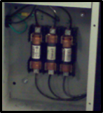
All objects on earth emit infrared (IR) radiation. Through the use of non-contact infrared cameras, a certified thermographer can detect and measure IR radiation emitted from a surface and measure surface temperature and thermal gradients. Figure 1 shows how thermal imagers easily detect important phenomena that the human eye cannot.
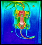
Figure 1: Dangerous condition in electric fuse
An infrared camera is an electro-optic device composed of a detector, IR optics, display, controls, storage media and power supply. See Figure 2. These instruments have many industrial applications providing the user with visual displays of thermal patterns and quantitative data that can be analyzed with either the manufacturer’s image analysis software or statistical software like JMP.
Figure 2: Fluke Ti32 thermal imager
Of particular importance are the detector and the optics. Typical detectors are sensitive to radiation in two spectral bands, mid-wave IR (2.5-6.0µm) and long-wave IR (8.0-15.0µm). The focal-plane array detector comes in a variety of resolutions. For the Fluke Ti32, the array is 320 x 240 pixels, considered to be high resolution for thermal cameras. A single image thus yields the same information as one would get from 320x240=76,800 discrete thermocouples. The detector size and density combined with the optics establishes the system’s spatial and measurement resolution.
Heat marches to its own drummer
Energy leaving a surface may be comprised of emitted, reflected and, for some materials, transmitted electromagnetic radiation. For thermographic analysis, only the emitted energy provides useful surface temperature information and compensation must be made for reflected and transmitted energy, if present. Fortunately, a certified thermographer knows these limitations and can use the imager’s algorithms to sidestep the unwanted influence of reflected energy, background energy and the IR transmission inherent in certain materials. It is critical to note that IR cameras have a substantial learning curve and that about a week of hands-on training is needed to assure accurate measurements.
Emissivity is a key property that describes a material’s ability to give off (emit) thermal radiation. Emissivity varies between 0 and 1 and is a function of material type, surface condition, temperature, wavelength and angle of view. Again, the skill of the certified thermographer plays an important role in assessing the object under study and setting the imager to make dependable measurements.
Thermography, it’s not just for building inspections anymore
A wide variety of applications exist for infrared thermography including electrical, electromechanical, mechanical, building & roof diagnostics, nondestructive testing, aircraft inspection, industrial process control and industrial process improvement. Many applications exist in the plastics industry including thermoforming, as discussed in this paper, as well as extrusion, roto-molding and injection molding.
The Fluke Ti32 imager
The Fluke Ti32 imager used for this process improvement project has a microbolometer detector array that operates in the longwave infrared spectrum. The Instantaneous Field Of Viev (IFOV) for this system is 1.25mRad and the minimum focus distance is approximately 6 inches with the built-in lens. The thermal sensitivity of this model is very good at 45mK and the acquisition rate is 60Hz.
Images in this report were processed and analyzed utilizing Fluke SmartView® software. This software includes various analysis tools, the adjustment of variables like emissivity and the export of data. The software allows the thermographer to retroactively change all camera adjustments except, of course, for the focus.
IT’S ALL ABOUT THE HEAT
Engineering knowledge points towards temperature control as a critical factor during all phases of the thermoforming process. It is a well-established fact that good parts are a result of even heating and cooling of both the plastic blank and the thermoformed part. Excessive thermal gradients are known to cause part distortion, poor thickness control, structural weakness and poor surface finish.
THE CHALLENGE
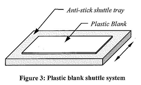
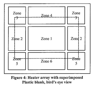
The thermoformer oven under study has an unusual design with a shuttle system and single-sided heating array as shown in Figure 3 and Figure 4.
The shuttle tray is on rails that move the plastic blank directly under a multi-zoned horizontal heating array and then shuttle-out the heated blank where it is picked up and vacuum-formed by hand onto awaiting molds. Heating occurs from one direction only and the distance from the tray to the heater array is fixed. The array and superimposed blank is shown in Figure 4.
It was known from past studies that the surface temperature of the blanks varied significantly along its length and width. One operator remarked that the first exploratory thermal image of the heated blank looked like a Jimi Hendrix tie-dyed shirt from the 1970’s!
The work contained nothing new experimentally, so the remainder of this paper emphasizes the step-by-step approach to experimentation, team dynamics and the experimental philosophy used for decisions.
EXPERIMENTAL TEAM
Company management chose 3 people for the work – a skilled Line Operator (a customer!), a Supervisor and a Process Engineer with DOE experience. Other people were brought into the work as needed. Hereinafter, this group is referred to collectively as the experimenters.
DOE PHILOSOPHY
Despite its technical slant, DOE success depends on the philosophical underpinning of the experimenters and their managers.
DOE is iterative
Despite the corporate designation of the thermoformer process study as a discrete Approved Project with a target end date and various milestones, the experimenters stealthily thought along different lines. They saw the work as the beginning of numerous, preferably brief, cycles of learning1,2,3,4 that would yield in depth process understanding. They were not after a quick fix.
DOE is not a spectator sport
Those with previous DOE experience knew that it’s usually preferable to run the experiment and collect the data themselves rather than hand the task over to a lab technician or other colleague. Therefore, all experimenters planned to get their hands dirty, whether they wanted to or not.
Beware of assumptions
Everyone agreed to take nothing for granted. They carefully observed the process, made notes, spoke with operators and eventually ran the process themselves. Experimenters did the weekly maintenance checks, controller self-test and the like. A few issues were discovered and addressed prior to the start of the work. In the end, there seemed to be a strongly positive correlation between knowledge gained and the amount of grit on the experimenter’s hands.
STEP 1 – ESTABLISH THE GOAL
Many industrial experiments fail because the goal is not carefully defined. A useful document titled Checklist for Asking the Right Question5 provided a lean, simple solution to this potential problem and a superb forum for group discussion. In time, the group reached an unusual consensus - the existing knowledge base was too sparse to state the goal in a typical managerial way like reduce scrap by 25% in 6 months or increase uptime by 5% every 2 months. Instead, the goal was defined non-traditionally, in the form of a target condition3 as shown in Figure 5.
INCREASE PROCESS UNDERSTADING
WITH MAXIMUM OPERATOR INVOLVEMENT
AND ITERATIVE DESIGN OF EXPERIMENTS
Figure 5: Target Condition
It was believed that improved process understanding across all organizational levels would lead inexorably to useful predictive models and new knowledge. Then, they’d be equipped to determine the ideal duty cycles of each heater zone and production practices for a wide range of plastic types, size and thickness.
STEP 2 – CHOOSE A STRATEGY
The experimenters had to decide between the 3 basic approaches to experimentation5:
- Screening
- Interactions model (frugal)
- Response surface model (thorough)
With the painful history of unpredictable thermoformer performance in mind, company management approved ample resources for the experiment and the group quickly agreed on the response surface approach.
STEP 3 – CREATE A PLAN
Strategy in hand, everything was in place to create a plan.
Choose experimental factors & ranges
The plan had 6 process factors - the duty cycles, in %, of each heater zone. The ranges varied from 20-60% to 30-70%.
Think about known factors to hold constant
Factors that were not under study were held constant during the experiment.
- Machine operator (an experimenter)
- Production lot of plastic blanks
- Time between ejection of heated blank and the capture of the thermal image
- Etc.
Danger, lurking variables!
The project team spent most of their time in the work area, providing a fine opportunity to identify and address a long list of insidious lurking variables.
- Ambient temp
- Ambient humidity
- Air circulation
- Time of day, breaks
- Etc.
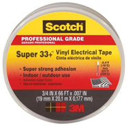
The plan included a thermoformer warm up time of 1 hour to assure steady state thermal conditions, the recording of lurking variables and doing the experimental runs in succession, without breaks. One thermographer trick was particularly useful7. The experimenters placed Scotch® Super 33+ black vinyl electrical tape on a non-metallic object adjacent to the thermoformer. See Figure 6.
Figure 6: A thermographer’s best friend
This tape has a predictable emissivity of 0.95 and it provided an excellent measurement point for ambient temperature. Krylon flat black spray paint also has an emissivity of 0.95 and can be used for the same purpose7.
Choose responses
The initial plan had one response and the experimenters were open to adding more as they accumulated new knowledge. This was yet another departure from the historical approach to planning everything in advance and stating arbitrary deadlines. Their alternative approach - add new responses as mounting new knowledge indicates - cost little and revealed much.
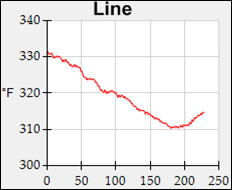
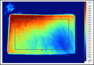
The original response of interest was the thermal gradient in the plastic blank. Here is where the advantage of radiometric data pays huge dividends. When the image is saved as a radiometric data file (.is2) Fluke’s SmartView software can export the actual data array (76,800 data points) or a subset thereof to a .csv file. Then, the experimenter is free to define the response variable as needed. For example, it could be a measure of the distinct thermal gradient along an indicated line as shown in Figure 7 and Figure 8.
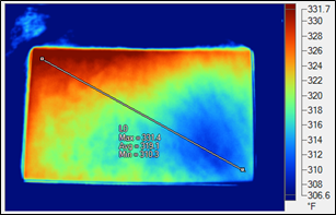
Figure 7: Thermal image with line of interest (L0)
Figure 8: Plot of surface temperature along L0
Or, the response could be the thermal gradient within a rectangular area. See Figure 9.
Figure 9: Thermal image with area of interest (A0) and surface temperatures
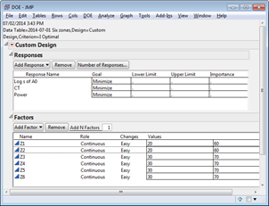
Either the line or area response is vastly superior to using readings from a discrete thermal gage as the experimental response. The experimenters chose log s of Area A0 as their thermal gradient response variable. Two more responses were added later - the measured process cycle time in minutes (CT) and the calculated power consumption. These responses have important financial implications in the form of plant throughput and energy costs. Figure 10 summarizes the final plan.
Figure 10: Factors & responses
Define model & plan replicate runs
At first, it was thought that a 6-factor experiment would result in an unmanageable number of runs, but with a short heating cycle and low material costs, the project team decided on a full quadratic model, minimum plus 4 runs and 8 replicate runs as shown in Figure 11. With clever planning, experimenters could run all 40 trials in one day, hence no blocking was needed.
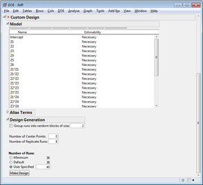
Figure 11: I-Optimal Design
Design Check
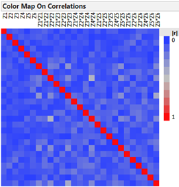
The Color Map on Correlations showed that the design was good and the experiment could proceed. See Figure 12.
Figure 12: Design check
Philosophical note on team dynamics
Thermal images like those shown above, the easily understood DOE design screens and the JMP Fit Model output shown below drew much attention from experimenters and other factory personnel. During the work, thermal images were taken of objects, machinery and people and their meaning was enthusiastically discussed. Meanwhile, the JMP Prediction Profiler and Interaction Plots triggered much discussion and lively debate. Opinions were stated. Experience was shared.
As a result of these remarkable team dynamics, people freely chose to participate in the process improvement effort, thus proving the lean adage keep it simple and visual.
STEP 4 – EXECUTE THE PLAN
As usual, a few practice runs were in order to work out the expected procedural kinks. Adjustments were made to the document titled Checklist for Asking the Right Question and clear operational definitions were written for all measurements. Then, the experimenters got their hands even dirtier collecting the 40 sets of response data. Much was learned along the way.
Pre-requisite #1 - check for constant s
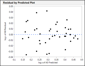
After fitting the collected and calculated response data to the model, the results were checked for constant s using 3 visual methods, the residuals-by-predicted plot, the Box-Cox plot and a normality check of residuals. Two of 3 passed the test (see Figure 13 for an example) and the team proceeded to the next pre-requisite.
Figure 13: Check for constant s
Pre-requisite #2 - measurement sanity check
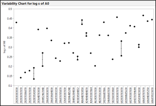
With 8 replicate runs, it was possible to check the repeatability of the process and measurement system. JMP’s tabular EMP output6 (Figure 14) revealed that 90% of the measured variation came from the experimental runs themselves. JMP’s Variability Chart (Figure 15) provided corroborating insight in graphical form.
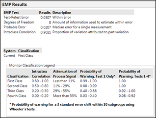
Figure 14: EMP sanity check
Figure 15: Variability Chart
These results were easy to understand and the experimenters agreed to proceed.
Review results
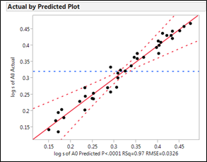
JMP’s Fit Model output is highly graphical in nature, easing the task of explaining experimental results to people at different organizational levels. The output ranges from tabular to graphical to highly interactive as shown in Figure 16 to Figure 19.
The Actual by Predicted plot (see Figure 16) is an assessment of the quality of the model itself. The plotted points indicate good predictive ability.
Figure 16: Actual by predicted plot
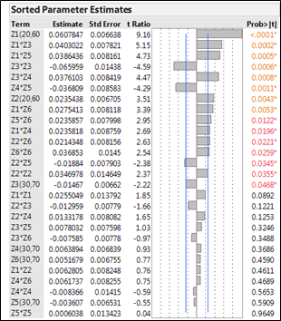
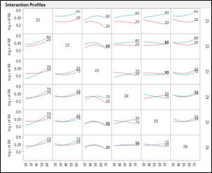
The Sorted Parameter Estimates (Figure 17) tell us, in a concise tabular/graphical form, the relative significance of each term in the model. The most significant factor was the main effect of Zone. The second and third most significant terms are the Zone 1-3 interactions and the Zone 1-5 interactions. The Interaction Profiles (Figure 18) provide additional insight.
Figure 17: Sorted parameter estimates
Figure 18: Interaction profiles
The discovery of the strong Z1-Z3 and Z1-Z5 interactions (i.e. those with corner-to-corner juxtapositions) was a quantum leap forward in process understanding.
Pondering and choosing a sweet spot
The experimenters and company executives found the JMP Prediction Profiler allows clear visual assessment of technical-financial tradeoffs, providing an easy, powerful way to make business decisions based on data from actual process observations. See Figure 19.
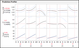
Figure 19: Prediction Profiler
Some of the heating zones did not have a dramatic impact on thermal gradients, so the duty cycle could be set toward the low end of the range to save on power costs, to extend the lifetime of the heating elements, to save on maintenance costs and to reduce costly production interruptions.
There is nothing wrong with your designed experiment…
As nature abhors a vacuum (well, at least here on earth, anyway), some manufacturing people likewise abhor the area near the extremes of the experimental ranges and steep areas of the response curves. As a result, the team pondered the experimental Outer Limits with caution as they knew nothing about what happens at duty cycles outside the tested ranges. For example, what would happen if Zone 1 drifted to a duty cycle of 65%? Nobody knew.
Conversely, when response curves are steeply sloped, as was the case with Zone 3, abhorring-the-extremes can be costly. A small change in the factor can trigger a significant change in the response. Note that the minimum value of log s of A0 occurs at a duty cycle for Zone 3 of 70%. However, that set point is at the extreme of the tested range and on the steep part of the Zone 3 curve, a Process Engineer’s worst nightmare. Figure 20 highlights this process danger zone.

Figure 20: Pesky Zone 3
The experimenters decided to reduce the Zone 3 duty cycle to 41% and accept the resulting penalty in log s of A0. The rationale: choose process settings that are robust to sources of variation like aging of the heating elements, ambient air currents, drift, error, etc. Figure 21 visualizes the rationale behind the chosen sweet spot for all 6 zones, again in the center of a plateau, away from the extremes.
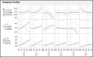
Figure 21: Manufacturer’s Heaven
Test model and evaluate tolerance interval
Next, the experimenters repeatedly tested the sweet spot and used the accumulated data to calculate a tolerance interval, in this case with 95% confidence on 99% of future product. The tolerance interval proved satisfactory vis-à-vis customer expectations.
STEP 5 – ACKNOWLEDGE SUCCESS
With the powerful new knowledge gained during the experiment, the experimenters confidently recommended permanent changes to company management. Action was taken. Additional study was approved. However, a few important matters remained.
Reflect
The experimenters learned from their mistakes. A lean practice, Hansei9, suggests reflecting upon work methods after reaching a significant milestone like the end of one cycle of learning and the beginning of another. The team had an informal and honest discussion of what they did wrong and what they could have done better. This exercise proved useful for follow on studies and future experiments.
Help others
The experimenters also took the time to engage in another useful lean practice, Yokoten10, which suggests lateral sharing of best practices across the organization. The benefits of this practice include introducing DOE methods to others and helping them perform their own experiments.
Acknowledge
In addition, the team paused to acknowledge their success and made sure that all participants were visibly recognized for their contributions. Large stacks of pizza pies were brought in.
Monitor
Additional log s of Area A0 data were collected regularly to detect the presence of process drift. Should the oven performance deteriorate significantly, the problem would be quickly visible and then investigated and addressed.
KEYS TO SUCCESS
The quality of the results attained were greatly influenced by the superb contributions of front line workers, the use of JMP’s vaunted data visualization capabilities, the ability to “see heat” and a consensus approach to decision-making. It also was clear that Design of Experiments and thermography are highly complementary technologies. Had the team been limited to trial & error, one-factor-at-a-time experiments or the use of discrete thermal gauges, the thermoformer would almost certainly have continued limping along as it always had.
OTHER APPLICATIONS
Experiments with thermographic response variables can be used wherever manufacturers require knowledge of process cause and thermal effect. Following are a number of different applications where thermographic response variables would prove useful. Many more are sure to exist.
- Food manufacturing
- Extrusion
- Annealing & heat treating
- Metallurgy
- Injection molding
- HVAC design
- Composites
- Pultrusion
- Heater, cooling system and dryer design
REFERENCES
[1] Roger Hoerl and Ron Snee, Statistical Thinking, 2nd edition, John Wiley & Sons, The Wiley and SAS Business Series, 2012
[2] Ian Cox, Marie A. Gaudard, Philip J. Ramsey, Mia L. Stephens and Leo T. Wright, Visual Six Sigma, SAS Institute, Inc., Published by John Wiley & Sons, SAS Business Series (2010)
[3] Mike Rother, Toyota Kata, Ch. 5, McGraw-Hill, 2010
[4] The Shingo Institute, The Shingo Model, Utah State University, 2014
[5] William D. Kappele, Performing Objective Experiments Using JMP, 5th edition, August 2011, Objective Experiments. Checklist is available at www.objexp.com.
[6] Donald J. Wheeler, EMP III, Evaluating the Measurement Process, SPC Press, 2010
[7] The Snell Group, Level 1 Thermography Course Manual, Barre, VT, 2014
[8] Juran’s Quality Handbook, Chapter 6, Juran and DeFeo, McGraw-Hill, 2010
[9] Gemba Academy Blog, Repent, I Mean Hansei!, May 2, 2007
[10] Gemba Academy DVD, JIT Technologies, Part 6
ACKNOWLEDGEMENTS
Bill Kappele of Objective Experiments provided key review and commentary on this paper.
AUTHOR BIOGRAPHIES
Stephen W. Czupryna is a Process Engineering Consultant and Instructor with Objective Experiments in Bellingham, WA. He has a B.S. degree in Economics, an A.S. in Laser Electro-optics and is a Pyzdek Institute certified Lean Six Sigma Black Belt. He also has a Level I Thermography certificate from The Snell Group with acknowledged competency in both electrical and mechanical IR testing.
Tony Shockey is the Fluke Thermography Services Manager for the America’s. He comes from industry and has a background in Instrumentation, Automation and Process Control from Bellingham Technical College as well as Infrared Level II – ASNT compliant training. As a Subject Matter Expert at Fluke for 7 years, he’s presented worldwide on these subjects, performed extensive training to channel partners and key end users and continues to be back line technical support for Fluke Corporation.
Roy Huff is Vice-President of The Snell Group. He teaches and consults in a wide range of infrared and electric motor testing subjects. Roy holds a BSEE from University of Missouri-Columbia and a Level III Thermal/Infrared certificate from ASNT. He is certified by SMRP as a Certified Reliability Maintenance Professional and holds Level III IRT NAS410 certification. He has presented at P/PM National Symposium, Thermosense, Thermal Solutions, EPRI, SMRP and other conferences.
Discovery Summit 2014 Resources
Discovery Summit 2014 is over, but it's not too late to participate in the conversation!
Below, you'll find papers, posters and selected video clips from Discovery Summit 2014.
- © 2024 JMP Statistical Discovery LLC. All Rights Reserved.
- Terms of Use
- Privacy Statement
- Contact Us
