Hi. Thanks everyone for joining us.
The title of this presentation is Choice Design and Max Difference Analysis
in Optimizing a High School Laptop Purchase
in the Context of a STEM project or STEAMS project.
My name is Patrick Giuliano.
I am a co- author and co- presenter for this presentation.
And of course, this is JMP Discovery Summit Europe 2022.
And I'm happy to be presenting today.
So before I get into our project definition or project charter,
I just wanted to mention some general context for this project.
So this project has a STEAMS orientation, which is basically a STEM framework,
but with the addition of a focus on practical AI and statistics,
and through the lens of JMP.
All right. So the opportunity statement for us here
is that every year, students in grade nine
with respect to Stanford Online High School,
they need to take core courses and need to do a series of projects.
In fact, there are many projects per year, as many as 150,
and many of them require the collection of survey data.
So in the context of survey data collection,
JMP has a powerful Choice Design and choice modeling platform
as well as Max Difference design capabilities, and those can be used
to optimize both survey methodology and analyze survey data.
Within this particular use case, we're going to use JMP 16 Choice Design
choice modeling platforms to study consumer research,
and also specifically to assist with the choice of a laptop,
the optimal choice of a laptop for a student.
We're going to also take this a step further
and look at some reliability questions and do some calculations
to look at the opportunity costs associated with purchasing a warranty
at different stages of ownership.
All right. So quick orientation to our STEM diagram here.
We had ten respondents in the context of our example, our sample data set.
In fact, this is a JMP sample data set, which I will provide on the user community
and is also available in JMP Sample Data directory.
There is ten respondents in this survey.
As you can see here in the lower left hand corner of the slide,
there are four attributes that change within a choice set.
There are two profiles per choice set. There's eight choice sets per survey,
one survey total to be distributed, and of course, ten responses as we indicated.
So in terms of the technology associated with the laptop,
we're looking at four key attributes.
We're looking at hard disk, drive space,
processor speed, battery life, and the computer cost.
And we can see a picture of the design as well as the different choice sets
that are paired by number with the different attributes in the columns.
And then, quite nicely, we see a probability profiler
which really just shows the opportunity space
in relation to the changes in the axis across the four parameters on the right
result in a change in probability or likelihood of purchase.
Okay. So let's provide an orientation
to the science and the statistics with respect to consumer research.
So we're going to think about collecting information,
and we want that information to somehow reflect how customers
use their particular products or services in general.
We want to have some understanding of how satisfied customers are
with their purchase and what features they might desire.
What insights they can use to improve the problem statement that
they're working on in the context of the purchase that they're making.
In this project, we use JMP's Consumer Research menu,
and specifically, we're going to focus on the Choice Design platform.
Okay, so here are some nice graphics that just show,
that highlight the consumer research process.
And like many processes, we can see that it's very iterative and cyclical.
It's focused on strategy development,
decision making, improvement, and solving challenges.
But as we'll see later in the analysis, there are specific modeling considerations
that Choice Design takes into account
to make our modeling procedure a little bit simpler and more effective
for these particular types of problems.
All right, so going back to our overview of the study.
So the voice of the customer really speaks to how the manufacturer
decides to construct the design in our case.
And so we have two sets of profiles,
again, that will be administered to ten respondents.
And the goal is to understand how laptop purchasers
view the advantages of a collection of these four attributes.
All right. So our particular use case here
is going to be the Dell Latitude 5400 Chromebook.
This is a very common budget laptop
that would be considered appropriate for student usage.
Okay, so here's an overview of the Choice Design modeling platform.
We can see that the four parameters are specified under the Attributes section.
HDD size, processor speed, battery life and sale price,
and the high low levels of the design are specified
over at the right under Attribute levels.
So you can see that by generating this design,
JMP gives us a preview of the design and the evaluate design platform
with our choice sets, and our hard drive stays,
our disk size, our speed, our battery life,
and our corresponding price for each of the choice sets,
where the choice sets represent a choice
between one computer possessing a certain set of features and another.
So as I mentioned before, we're going to bring in the sample data
and actually point to the specific location where the data is located.
We're going to go ahead and put that in the community
for our users to practice with this data.
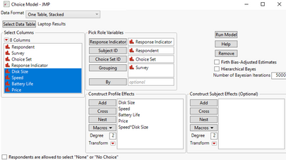
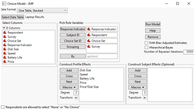
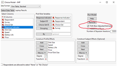
Okay.` Here is the display of the model specification window for Choice Design.
So after we've generated the design, we have to fit the design.
And so we can see that the structure of a design is ten respondents that are paired.
And so we're going to set the data format to one table, stacked.
Our select data table, it populates into the Laptop Results Data table.
Our response is related to probability of purchase, which is related to price.
We put subject into subject ID,
choice set in choice set ID, responding and grouping.
We cast our four attributes into the X role here.
And then we have a subject effects,
or we can have subject effects, which are optional,
which we didn't consider in this particular context that we can have them.
And we also have an option for missing value imputation, which is nice.
One of the things you'll notice here, though, is that
if you're familiar with JMP, you'll see that the run model option is here,
but there are no other options and in many other modeling platforms.
In JMP, we have what's called personality selection.
In this particular context,
we're limited to a specific model under a specific framework only.
Why is that?
Well, from our perspective,
this is likely because this modeling strategy
is very specific consumer research, and we would really only want to consider
main effects between choices because those effects reflect
the choice modeling structure that we're implementing.
We pick from either one set of features or the other.
Okay. So principally,
what a mathematical model or what statistical model
is underpinning this type of procedure?
It's really a logistic regression type model
because our wide response is a probability.
Our response can be thought of as whether we're going to make a purchase or not,
and therefore is the likelihood of making a purchase.
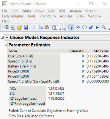
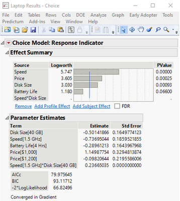
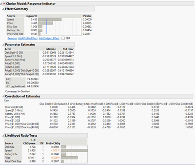
And so what we see in the summary of the model output
is that a negative estimate on the terms in the model indicates
that the probability of purchasing chance
is lower at that particular attribute level.
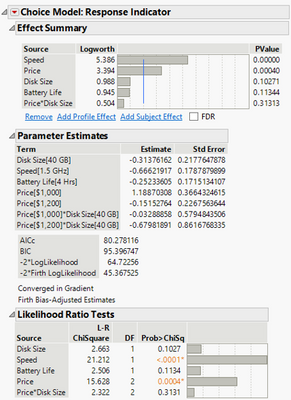
And so we can see from the summary, the parameter estimates
and from the ranking of the effects summary,
and that buyers generally prefer a larger hard drive size,
faster speed, longer battery life, and the cheaper laptop.
And we can see that speed and price
are really the most significant predictors on probability of purchase.
And we spoke a little bit on the buyer side
about why there isn't an interaction term.
We think that it's really because in the context
of this research problems, it's not really a practical consideration.
But certainly, it's not likely due to lack of degrees of freedom
because in this particular data set,
we had over 100 observations and we're only fitting four terms.
Okay. So another thing to notice here,
I think, that's not immediately obvious on the slide is there's
some discussion or notes at the bottom of the primer estimates
that say converged in the gradient.
And that just really speaks to the fact that this model estimation procedure,
this likelihood- based modeling procedure is an iterative procedure.
It's not necessarily deterministic,
and it involves iterating to find an optimal solution.
Okay. So let's take a look at the effect marginal analysis
and the context of this report.
So we can see here that the report shows marginal probability
for each of the four attributes that they're different levels.
And so what I'm highlighting here is that the marginal probabilities that are
the most different from each other indicate where there's the most
differentiation in terms of making the purchase decision.
So clearly, price and computer processing speed
are the most important in terms of really driving that probability decision.
And so as an example here, you can see that 71% of buyers
may choose an 80 gigabyte over 40 gigabyte hard drive size,
as indicated by the marginal probability of .7129,
and 68% of buyers may choose, for example, $1,000 over a $1,200 or $1500 price.
So that's indicated by the .6843 in this marginal probability.
So we can look within each of these marginal probability panels
to look at what the preference would be on the basis of a given factor,
like price or speed, and also look across the effect marginal panels,
and specifically look at the differences
in marginal probability or marginal utility
to see which factors are most differentiating
in terms of driving the purchase decision.
Okay.
So the next thing I'm going to talk about is the utility profiler.
So in addition to the response probability or likelihood of purchase,
we also have something called utility.
And so utility is really
something like probability, but it's defined differently.
And the utility profiler report shows, in effect,
a measure of the buyer's satisfaction at a particular scenario.
In the context of utility, a higher utility indicates
higher happiness, if you will; and a lower utility, below zero,
for example, indicates relative unhappiness.
And so we can see from this profiler that the utility is increased.
Or if you will maximize when purchasers spend the least amount,
they have the longest battery life, the highest processor speed,
and the largest size, which is completely intuitive in this context.
And what we can do is we can think about utility very much like we can think
about desirability in the context of traditional experimental design,
where we want to maximize this utility function
in order to maximize the buyer satisfaction.
And so as I mentioned here,
there is a relationship between probability and utility.
Mathematically, what is it?
Well, we don't get into that here,
but it is articulated in JMP's documentation.
And this is something that I'm going to be thinking about
as part of the dialogue to this talk when it's archived in the user community.
So look forward to that.
Okay. So now, let's look at the probability profiler.
So the probability profiler is going to be similar to the utility profiler,
as I discussed in the prior slide, but it's, of course, a little bit different.
So what is it, practically?
Well, the profiler set at these particular settings of X,
the response probability is 12%.
So the way we can interpret this is we can say that 12% of buyers
would consider to spend $1,500 to get a laptop with a 40 gigabyte disk,
1.5 GHz processor and a four hour battery life.
Okay.
So the way we like to think about this is that for any special condition
that you want to know what the probability is at a specific set of factor levels,
the probability might be more useful than, for example, utility,
which describes a measure of the buyer's overall satisfaction.
And you'll notice clearly that the profiler is limited to just two levels.
And again, this goes back to the nature of choice design and consumer research.
And we really want to h one in on the buyer's interest
by giving them a successive series of dichotomous choices to choose between.
Like how when we're at the optometrist, the optometrist does the lens flipping
and says "Is A better or B better?" A or B and then you go on to the next one,
and then she asks for a similar selection between A or B.
Okay, so the next part of the project is really around warranty consideration.
So I spoke about this a little bit in the beginning.
So let's go into this in a little bit more depth before we conclude.
So suppose the optimal choice for the consumer
was a laptop sold at a price of $1,000.
Suppose that the consumer purchased an extended warranty protection plan.
If they were to purchase one for two years duration,
it would be $102 and for three years, it'd be $141.
One of the key questions for the consumer is, well,
after they buy the laptop, do they buy the warranty as part of the purchase
right after the laptop or the extended warranty,
or do they wait, or do they just not buy the warranty at all?
And I think it's pretty obvious to everyone
that if you buy a higher price laptop, your warranty is going to be
a higher price more often than that.
So this is also a consideration in terms of making the final purchase decision.
We didn't necessarily incorporate in this hypothetical experiment.
Okay. So this slide just goes into a little bit more detail about warranty.
There's a lot of information here and I'll let our audience take a look at it later.
But a lot of this comes from our typical computer manufacturers website, like Dell.
And like anything, there's a lot of language
that is specific to an original limited warranty
and different terms and conditions that are associated with the warranty.
Some things that I think I should highlight
are this idea of onsite services.
The fact that more and more now, we have services where a service provider
will come to you and do repair or exchange of the product at your location.
There's also the customer carry-in and mail-in services, very popular now.
Even within the context of Amazon, mail-in services been around for a long time.
Customer carry-in is now a part of Amazon's ability to provide service
in the context of going to, for example, a Whole Foods Market for return.
And then, of course, product exchange.
But these onsite service models and mail-in service models
are very interesting and much more common today.
The other thing worth highlighting is that limited warranty services
depend on how you purchase your original warranty policy.
So if warranty services are limited,
those services are stipulated in the original warranty policy.
Okay.
So let's talk a little bit about the JMP's reliability and forecasting.
So in the context of this particular analysis,
we're going to use the life distribution platform in JMP
to do some reliability and forecast calculations.
And what we're going to try to do is predict future failures
of components or that be into the computer as a system
to help us get a better sense of whether we should purchase a warranty
and at what time in the life of the product.
So we can think of this analysis in terms of what we call reliability repair cost.
So we want to compare with the extended warranty protection.
We want to compare the ready initial warranty
to the extended warranty protection.
And of course, if the failure rate is too high,
then we won't want to purchase warranty protection at all.
And if the failure rate is very low, then there would be no need as well
for us to purchase any warranty
because we would have a product that lasted for a long, long time.
You can think of each product or each computer, in this case,
has its own unique reliability model.
And it's something to think about in this context.
So if you've made a particular purchase in this hypothetical scenario,
you can construct a reliability model on the basis of this particular computer.
Okay. So this slide talks about a nice visual representation
of a reliability lifecycle, if you will,
or failure rate over time for a particular product.
So we basically have three phases.
We have a startup and commissioning phase,
which is like a burning phase for a product.
Then we have a normal operation phase,
and then we have an end of life phase.
And so these phases can be, we referred to them sometimes
as the first phase, the running phase or the burning phase,
like the infant mortality phase in the context of survival for life.
For clinical studies, the normal active operation phase
can be thought of as the phase where random failures may happen,
and the end of life phase is really like the wear- out period,
the period before the product completely wears out in sales.
And so corresponding to these periods,
we can consider a general range of limited warranty over time,
and then a transition phase somewhere where that limited warranty
becomes an extended warranty protection policy.
So where we go from a short term warranty, maybe a year,
to a long term warranty, two or three years.
So like we said, if the failure rate is very low,
then perhaps if the product is expected to last more than two years,
then maybe you don't need a warranty policy
because you may plan to replace a product like this every two years
because it's just technology and opportunity cost of price
versus the benefit of new technology.
So the important thing to think about again in the context of making
the initial purchase is looking at the startup and commissioning of a product.
If we purchase an original warranty, which is what we commonly do,
it usually covers maybe a year of service
and it's part of the initial purchase of the product.
Okay.
So now, what we're going to do
is we're going to switch over to a different data set.
This is also sample data which will point you to on the community.
But we're going to assume that we have a database related to the Dell laptop.
And it lists the return months, the quantity return,
and the sold month over on the right.
And so what we can do is we can graph this information.
And the X is referred to the failure rate.
The X is in the space of an asset for the failure rate,
the reliability model, and how many parts we shipped.
That's what these three variables speak to.
And based on this probability, we can calculate
if they purchase the warranty policy or not against the repair cost.
How do we choose a warranty policy based on the failure rate or return rate?
So we can use the JMP's reliability forecasting capabilities to do this.
So here's a picture of the model that we use to fit this data.
So we have a probability on the Y axis, first time in months.
And what JMP does is it applies multiple models.
So we fit all available models at least once that were non- zero,
that were not producing non- negative estimates.
And what we can see here is the ranking of potential models
to fit this reliability data.
And so Weibull is the top choice here based on the AICc,
BIC, and negative 2 Likelihood ranking.
So we went ahead and went with the Weibull for our analysis, subsequently.
Okay. So here's an upper left hand corner of the slide.
What we see is the actual Weibull failure probability model fit with its parameters,
with primary estimates for beta, Alpha, scale, and location.
And then the lower right hand side of this slide, what we did is
we estimated the probability of failure at specific months,
again, using JMP's reliability tools.
And so how do we tie this analysis into something practical?
Well, beta is a very important parameter.
Beta is a very important parameter for Weibull distribution.
So a beta less than one might indicate a product
that really doesn't survive phase one;
that initial where a burning phase that we showed in the bath tip curve.
So in that case, we want to buy a warranty at all.
A beta approximately equal to one that would be maybe a product
that's in the middle of that curve, that's in that steady state period.
In which case then, we wouldn't want to buy a warranty
necessarily anyway in that case either, because we have a very reliable product.
So we wouldn't necessarily want to invest money in a warranty
when we would expect to use it.
Only when the beta is greater than one, and you can see in this case,
it's significantly greater than one.
Do we really want to consider purchasing a warranty?
In this particular example, 1.6 being higher than 1.5,
probably indicates that the product is entering that wear-out period,
that third phase, the productive curve.
So if we look at this year, drawing on, say, an example of 35, 36 months,
our failure probability is maybe 20%.
So that's how we would look at this, right?
As you go over and you look at the time, what would the probability failure be
in the first two columns of the estimated probability output there?
In this particular example, it's not completely clear
whether we should purchase a warranty or not,
and we likely need more information.
If we had seen a beta that was in the three to four range,
then that would probably suggest
that we would want to purchase an extended warranty
because we would anticipate that wear- out would be inevitable.
In the next few slides, we're just going to derive a simple decision model
to go with this reliability analysis in the spirit of the choice analysis,
the choice modeling methodology that we applied in the beginning.
So the consumer decision model has to consider a number of factors:
survival probability at each month, failure probability at each month,
which are, in effect, the same thing.
And the market laptop value each month between one year and three months,
of course, price depreciation happens, and the monetary loss if not purchasing
the extended warranty protection if the repair is needed.
And then we want to compare that monetary loss
versus the expense of purchasing the warranty.
So there's like a cost benefit analysis or a risk analysis that we're making.
So we show here, in this slide again, the months after purchase,
and then we show the survival probability at a particular month,
survival probability of the prior month,
and then the conditional failure probability at that month.
And so we just use simple conditional probability to calculate that column
that I should have indicated with the two all the way over on the right.
And what we're doing here is we're using the previous Weibull estimate
at each month to calculate the conditional failure probability
at the subsequent months.
All we're really doing is using the Lag function to generate column one.
So it's just the difference between each survival probability in month,
let's say, 13 and it's prior month, 12, and 14, and 13, and so on.
And then we're just taking the survival probability of the prior month,
subtracting the survival probability at the current month,
times the survival probability of the previous month.
This is conditional probability.
Okay. So let's talk about the market laptop value, which is really
the second thing we discussed in this extended warranty protection slide.
So we can create a simple linear model
to model the declination of value over time.
And that's, in fact, what we did.
And the slope on that model, we use four points to calculate the slope.
And the slope on the model indicates the percent drop every month on average.
You can see the slope is about 1.3%,
so we expect about a 1.3% drop per month on average.
And note here that we only really care about the declination after 12 months
and beyond because the first twelve months are typically covered under warranty.
Okay. So how do we model the cost of not purchasing the extended protection?
Well, we can compare to a two year warranty policy,
failing at two years as the worst case.
And we can see that if we look at extended warranty protection plan
at two years versus three years, $102 versus $141,
we get a Delta of around $45.
Similarly, the cost if not purchasing the two year production plan is $48
at two years versus $95 at three years,
and so that difference is on the order of $40 to $50 as well.
So what this shows us is that there's maybe a $50 gap
between the warranty plan and the estimated cost,
and that may be attributed to the services and other fixed costs.
But really to make the best decision about whether to purchase a warranty or not,
we want to consider the cost of not buying a warranty in this framework,
and the magnitude of beta together
to make the best decision about whether to purchase or not.
Okay.
So this is nearly the end of our analysis.
And I wanted to just highlight one other thing here.
So we can use a forecast capability here
to show us how can we determine the return rate,
what resources do we need,
and a lot of that depends on the performance of service.
How good service is.
If we have too many returns, if we don't forecast,
we may not have enough technicians to do the work.
So this is the type of analysis where we're considering the producer.
This is from the standpoint of the service provider and the producer.
Whereas in the prior analysis, we are considering everything
from the perspective of the purchaser or the consumer.
So this is really a producer cost model.
If they don't purchase the warranty,
what's the labor cost, and what's the material cost?
So the labor costs to handle all the repairs,
and the material cost to replace parts for repair.
And so we can see that there's a slight upward sloping trend
on the long term repair forecast,
and that trend really tells us what the value proposition is.
So as a manufacturer, you may be making revenuein the beginning,
but then you may lose money in the long run
if you're doing significant repair work.
Or as I said before, you may not have the capacity
to do the repair work that you're obligated to do
because of the liability problems with the product.
Okay, so just to conclude here.
I just wanted to share an overall key learnings here of our project.
We use the STEM or STEAMS framework
to really break up this project into a number of different elements
and apply an interdisciplinary framework.
And we use Choice Design, and to help consider
survey design methodology as well as an analysis of survey data.
We also augmented our design with a reliability performance model
to qualify our purchase and whether or not that was a good purchase.
Of course, the project in the context of the co- authors, including Mason Chen.
Chen was very useful for motivating high school students at SOHS,
and teachers to learn new methods.
The final thing is one thing that we could consider in the future
is increasing the number of levels to choose from,
which would bring our model into more of a traditional modeling framework.
A modeling framework that's more like a lease regression model
or another particular popular modeling framework that looks continuous data.
And so in closing,
I just wanted to highlight our references and our statistical details;
we're going to definitely provide those to you.
Thank you very much for your time and I look forward to any questions.

