Regression Control Charting Using the Random Coefficient Regression Method
JMP® Discovery Summit Europe 2017, Prague
Pius Dahinden, PhD, Manager Analytical Science, Tillotts Pharma
Abstract
Since the new EU GMP Guideline (EudraLex Volume 4) Chapter 6 (Quality Control) took effect in 2014, performing a trend analysis on drug product stability data is an additional analytical quality control requirement. The European Compliance Academy's (ECA) Analytical Quality Control Working Group (AQCWG) has worked out a standard operating procedure for the assessment of out-of-expectation (OOE) and out-of-trend (OOT) results. For the assessment of stability data it is recommended to use the regression control chart (RCC) procedure for the comparison of current batches with data of historical batches. However, the slopes and/or intercepts estimated from the historical batch data themselves are subject to uncertainty. The ECA AQCWG proposes a simplified random coefficient regression (RCR) method which takes this into account. A newly developed JMP script which implements the recommended RCC / RCR procedure is presented. The script makes the identification of OOE / OOT points in stability data simple and provides all the necessary information in the output, together with an appropriate graphical display.
Introduction
Manufacturers apply statistical process control (SPC) to ensure the quality of the produced items and to prevent financial losses caused by production processes being out of control. Process control means that a running process is routinely monitored and that, if any of the monitored parameters should exhibit an anomalous trend, measures are taken to bring the process back under control. SPC is a tools that enables manufacturers to early detect changes in a process, allowing them to investigate trouble causing issues and take corrective actions at an early stage. A powerful tool for process monitoring is the control chart method which was popularised by Shewhart [6]. Figure 1 shows the schematic view of a typical control chart.
In contrast to production processes where there should be no trend, there are many data management problems with an inherent trend. For the analysis of data management problems of that kind the conventional control chart method has been combined with regression analysis, and this approach was referred to as the "regression control chart" (RCC) by Mandel [4]. As control limits the utilisation of tolerance intervals (TI) is reasonable. For monitoring stability data of pharmaceutical products stored at the recommended storage condition (e.g., 25 °C / 60% RH) RCCs are used to monitor, e.g., the degradation of the active pharmaceutical ingredient or the accumulation of impurities over time, to support the expiration dating of the product, i.e. to confirm the stability of the drug product for the duration of the labelled shelf life.
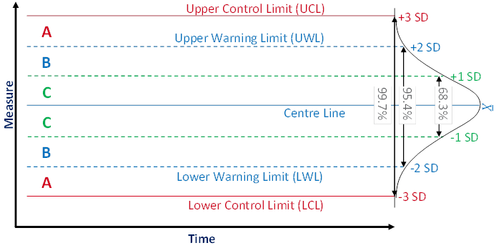
Figure 1 Typical control chart composition
A control chart usually shows the values or a statistic of several values (e.g. the mean) of the quality characteristic of a sample versus the sample number or the time. In general, the chart contains a centre line that represents the mean value of the in-control process. A fundamental assumption is that the data are normally distributed. Two additional characteristic horizontal lines are the lower and upper control limits (LCL and UCL, respectively) at a distance of ± 3 standard deviations (SD) from the centre line such that, as long as the process is in control, 99.7% of the data points will fall within these limits due to random variation which is denoted as common cause variation. The lines at a distance of ± 2 SD from the centre line are called the lower and upper warning limits (LWL and UWL, respectively) while the lines at a distance of ± 1 SD from the centre line don't have a specific name. By aid of these lines a control chart can be partitioned into zones C to A. Rules for the detection of special cause variation which characterises a process not being in control use the frequencies of observations in these zones as a decision basis.
Procedures and Results
RCC applied to stability data of a pharmaceutical product aims at answering two questions: 1) Is the current batch out of expectation (OOE) or out of trend (OOT) in terms of the historical batches (i.e. concerning the TI derived from historical data), and 2) is the most recently measured data point of the current batch OOE in terms of the current batch (i.e. concerning its prediction interval (PI))?
A minimum of three data points of the current batch are necessary for the assessment of a trend in terms of question 1. For the assessment of question 2 at least four data points are needed because the most recently measured data point should not be used for the construction of the PI.
Since it is very likely that the individual historical batches vary with respect to their intercepts and their slopes an ordinary least squares model (common slope – common intercept) might not be meaningful. For this reason the European Compliance Academy (ECA) Analytical Quality Control Working Group (AQCWG) recommends to make use of the "random coefficient regression" (RCR) method which accounts for the variability of intercepts and slopes of the individual batches [7]. A simplified RCR model (modified Carter and Yang [1] model) contains two unknown parameters, i.e. the intercept and the slope . This procedure is in accordance with WHO [9] and ICH [2] guidances.
The term OOT has been defined by the United Kingdom Medicines and Healthcare Products Regulatory Agency (MHRA) as a stability test result that does not follow the expected trend, either in comparison with other stability batches or with respect to previous results collected during a stability study [8]. The term OOS has been defined by the MHRA as a test result that does not comply with the pre-determined acceptance criteria or a test result that falls outside of established acceptance criteria which have been established in official compendia and / or by company documentation [8]. So far there is no formal definition of the term OOE. The ECA AQCWG proposes (for both qualitative and quantitative testing) to define OOE results as anomalous, unexpected or unusual findings that cannot be classified as either out of specification (OOS) or OOT [7].
RCR Model
The simplified RCR model can be written as
where is a vector representing the batch's repeated measurements (where , with representing the total number of repeated measurements of batch ) on the response variable (e.g. assay [%], sum of impurities [%] or dissolution [%]), and are vectors of the batch-specific intercepts and slopes, respectively, is the batch's time vector (e.g. [Month]), and is an vector of random errors. A prerequisite for this RCR model is a linear relationship between the response and the explanatory variable. If the relationship should be not linear an appropriate transformation has to be applied before performing the RCR modelling.
It is assumed that each comes from a univariate normal population with mean zero, variance , and all 's are independent of each other (conditional independence) and of the model coefficients and . This assumption is reasonable because it is highly improbable that the analytical method variability depends on the batch being tested or the point in time when the testing is executed. It is further assumed that each batch's regression coefficient vector, , is independent of their and all other batch's vectors of random errors, .
The RCR modelling comprises three steps.
Step a) Fitting a simple linear regression model to each batch's data
The data associated with batch are denoted by , where represents the batch's measured response at time point , where . The individual time points may differ between the batches, and so may the total number of time points . The design matrix for batch can be written in matrix form as follows.
This matrix is normalized and designated by .
The estimates for the intercepts , the slopes , the "Mean Square Error" of regression , and the degrees of freedom associated with are obtained by fitting a simple linear regression model to each batch's data. The intercepts and slopes are estimated by
.
Step b) Estimating the error variance-covariance matrix
Estimating the error variance-covariance matrix of the random coefficients starts by estimating the pooled of all batches, i.e. , as follows.
The numerator in this equation can be expressed as follows.
The sample variance-covariance matrix of the estimated intercepts and slopes is calculated as follows.
where , i.e. the mean vector of the coefficients, i.e. intercepts and slopes (ULS stands for "Unweighted Least-Squares"). Now, the variance-covariance matrix can be estimated as follows.
where , i.e. the mean model variance-covariance matrix. The error variance estimates the variance of the analytical method. The intercept variance component represents the within-batch variance of the response observed at product release due solely to the manufacturing process, i.e. excluding the variance which is due to the analytical method. The slope variance component represents the between-batch variance of the degradation rates.
Since the variance-covariance matrix is estimated calculating the difference of two matrices, the result may not be positive-definite, i.e. the intercept and / or the slope variance component(s) may be negative. One possible remedy to this is replacing the negative value(s) with 0. This is a simple first-aid approach for negative variance estimates and is equivalent to converting a random effect into a fixed effect. In case that both variances are zero the RCR model corresponds to the ordinary least squares (OLS) model.
Step c) Estimating the coefficient mean vector by a weighted least squares (WLS) estimator
The estimation of the coefficient mean vector starts with the calculation of the estimate of ,
which corresponds to the inverse of the variance of the regression parameter estimate for the batch. Based on this equation the dimensional matrix of the intercept and slope coefficient estimates, i.e. the weighted least-squares estimate, is now obtained by the following equation:
where is an estimate for the variance of the weighted least-squares estimator. The average of the intercept estimates represents the response at product release averaged over the manufacturing process, and the average of the slope estimates represents the common slope.
Tolerance Interval (TI) for RCR Model
The RCR model coefficients and describe the general trend, i.e. the common trend of the historical batches. The TI for the RCR model can be calculated by aid of the estimate for the regression line and its standard error according to the method proposed by Scholz and Vangel [5] as follows. Their method makes use of the effective sample size concept.
The error term is calculated by
where , and is the diagonal of the argument. The factor is given by
where the factor is the quantile of the t distribution with degrees of freedom and the non-centrality parameter , where is the quantile of the standard normal distribution. The parameter is the effective sample size given by
where the parameter and the variance ratio are defined by
where is the between-batch-variance, is the within-batch-variance (or method variance), is number of measurements per batch , i.e. , is the number of historical batches, and is the total number of samples, i.e. .
The TI covers of the population with a probability of . The effective sample size concept takes into account that the within-batch data are more correlated than the between-batch data which diminishes the amount of independent information. For this reason the following is always true: . The ideal case is realized if the within-batch data are totally uncorrelated.
Implementation of RCC / RCR in JMP
The JSL script implementing the RCC / RCR procedure is structured into several parts.
First of all the reference and test batch names and the various variable names for the response, the time, the batches and the storage condition have to be defined.
The RCR model is constructed (simplified Carter and Yang [1]) as outlined above.
The TI for the RCR model is constructed using the method proposed by Scholz and Vangel [5].
A report window is generated summarizing the calculated parameters in tabular and graphical form.
Example
For the assessment of the script functionality various data sets were generated for nine historical batches and one current batch. The following code snippet executes step a) of the RCR model fitting, i.e. the intercepts (a, ), slopes (b, ), (root) mean squares errors ((RMSE) MSE, ), degrees of freedom (df, ), and number of observations (n, ) of the historical batches are collected and stored into vectors of length .
For( i = 1, i <= n.refBatches, i++,
	fm = Fit Model(
		Y( :Eval( responseVariable ) ),
		Effects( :Month ),
		Personality( "Standard Least Squares" ),
		Emphasis( "Minimal Report" ),
		Where( :Batch == refBatches[i] ),
		Invisible
	);
	fit = fm << Run;
	fitr = fit << Report;
	a.i[i, 1] = fitr["Parameter Estimates"][Number Col Box( 1 )] << Get( 1 );
	b.i[i, 1] = fitr["Parameter Estimates"][Number Col Box( 1 )] << Get( 2 );
	RMSE.i[i, 1] = fitr["Summary of Fit"][Number Col Box( 1 )] << Get( 3 );
	df.i[i, 1] = fitr["Analysis of Variance"][Number Col Box( 1 )] << Get( 2 );
	n.i[i, 1] = fitr["Summary of Fit"][Number Col Box( 1 )] << Get( 5 );
);
For( i = 1, i <= n.refBatches, i++,
	MSE.i[i] = RMSE.i[i] ^ 2
);
Step b) starts with estimating the pooled MSE (MSE.pool, ). Subsequently, the mean model variance-covariance matrix (M.bar, ) is estimated, which is then combined with the sample variance-covariance matrix (S, ) to obtain the variance-covariance matrix (Sigma.hat, ).
ab.i = a.i || b.i; // Matrix of the intercept and slope vectors
S = Covariance( ab.i ); // Sample variance-covariance matrix of the intercepts and slopes
MSE.pool = Sum( E Mult( df.i, MSE.i ) ) / Sum( df.i ); // Pooled MSE
RMSE.pool = Sqrt( MSE.pool );
M.i = J( 2, 2, 0 );
For( i = 1, i <= n.refBatches, i++,
	dat << Select All Rows << Invert Row Selection;
	dat << Select Where( :Batch == refBatches[i] );
	x = dat << Get As Matrix( {"Month"} );
	x.length = N Row( x ); // Number of observations
	colReprIntcpt = J( x.length, 1, 1 ); // Column of 1 representing the intercept
	x = colReprIntcpt || x; // Design matrix of the OLS model
	M.i = M.i + Inverse( x` * x );
);
M.bar = M.i / n.refBatches; // Mean model variance-covariance matrix
Sigma.hat = S - MSE.pool * M.bar;
Sigma.hat[Loc( Diag( Sigma.hat ) < 0 )] = 0; // Replace negative values on the diagonal of Sigma.hat by 0.
In step c) the RCR model coefficients ab.hat () are estimated by aid of the following code snippet.
M.i = J( 2, 2, 0 );
W.i = J( 2, 2, 0 );
For( i = 1, i <= n.refBatches, i++,
	dat << Select All Rows << Invert Row Selection;
	dat << Select Where( :Batch == refBatches[i] );
	x = dat << Get As Matrix( {"Month"} );
	colReprIntcpt = J( n.i[i, 1], 1, 1 ); // Column of 1 representing the intercepts
	x = colReprIntcpt || x; // Design matrix of the linear model
	M.i = M.i + Inverse( x` * x );
	W.i = W.i + Inverse( Sigma.hat + MSE.pool * M.i );
);
Omega = Inverse( W.i );
ab.hat = Omega * (W.i * ab.i`);
ab.hat = ab.hat`;
ab.hat.bar = V Mean( ab.hat );
The next code snippet shows the construction of the TI for the RCR model according to Scholz und Vangel [5]. For the construction of the interval the average intercept and slope coefficient estimates stored in the ab.hat.bar vector are used.
utp = Associative Array( dat:Month ); // Unique time points
time.points = Matrix( utp << Get Keys ); // Vector with (new) time points for which the response is sought
n.new = N Row( time.points ); // Number of data points of the new data set
m.x = J( n.new, 1, 1 ) || time.points; // Design matrix
n = Sum( n.i ); // Total number of data points
df.th = n - 2; // Number of degrees of freedom if only fixed effects are allowed, i.e. if a "common slope, common intercept" model is appropriate.
df = df.th;
variance.ratio = Sigma.hat[1, 1] / (Sigma.hat[1, 1] + MSE.pool);
t.f = 1 / Sum( (df.i / n) ^ 2 ) - 1;
If( Sigma.hat[1, 1] == 0,
	df.eff = df,
	df.eff = 1 / (variance.ratio / (t.f + 1) + (1 - variance.ratio) / n)
);
// Calculation of the k.eff factor on the basis of the effective number of degrees of freedom.
k.eff = Sqrt( (n - 1) / n ) * 1 / Sqrt( df.eff - 1 ) * t Quantile(
	gamma,
	(df.eff - 1),
	(Normal Quantile( (1 - alpha) ) * Sqrt( df.eff ))
);
t.quantil = t Quantile( (1 - alpha / 2), df.eff );
y.hat = ab.hat.bar[1] + ab.hat.bar[2] * time.points;
LTL = y.hat - k.eff * Vec Diag( Sqrt( m.x * (Sigma.hat + Omega / n.refBatches) * m.x` + MSE.pool ) );
UTL = y.hat + k.eff * Vec Diag( Sqrt( m.x * (Sigma.hat + Omega / n.refBatches) * m.x` + MSE.pool ) );
In the last part of the script the results are prepared for displaying them in a report window. An example report is shown in Figure 2.
The results summarized by the report window allow answering the questions posed at the very beginning of chapter 3 as follows: 1) since the 18 months data point (i.e. the most recent measurement) of the current batch lies outside the TI fitted to the data of the historical batches it has to be concluded that the current batch is OOE / OOT, and 2) since the 18 months data point of the current batch falls outside the PI of the current batch it has to be concluded that the current batch is also OOE / OOT in terms of the current batch. The same conclusion would should been drawn already at the preceding time station although the 12 months time point falls within the PI of the current batch. However, since this point lies outside the TI fitted to the data of the historical batches the overall conclusion at the 12 months time station must have been that this is an OOE / OOT point.
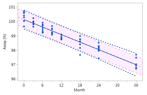
As mentioned at the beginning of chapter 3 it is very likely that the individual historical batches vary with respect to their intercepts and their slopes and that for this reason the RCR model outperforms the ordinary least squares model. Five cases can be differentiated: case I: no intercept variation, no slope variation; case II: intercept variation, no slope variation; case III: no intercept variation, slope variation; case IV: intercept variation, slope variation; and case V: non-linearity. The results summarized in Figure 3 for all of five cases. The graphs in Figure 3 show that the RCR model better represents the data in the cases where the intercepts and / or slopes vary and is very similar to the basic method in the cases where there is no intercept and slope variability.
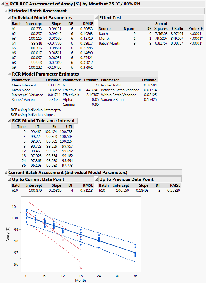
Figure 2 Output of script implementing the RCC / RCR method
The window is separated into the parts "Historical Batch Assessment", "Current Batch Assessment (Individual Model Parameters)" and the graphical display which summarizes the historical and the current batch data. The data from historical batches are represented by blue dots () and the data form the current batch by red crosses (). The TI fitted to the data of the historical batches is represented by the band delimited by the blue dotted lines and the PI fitted to the data of the current batch (but without including the most recent observation) by the band delimited by the red dashed lines.
I |
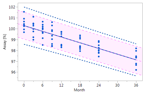 Figure_3_IIFigure_3_II Figure_3_IIFigure_3_II |
|---|---|
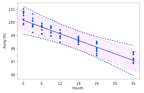 Figure_3_IIIFigure_3_III Figure_3_IIIFigure_3_III |
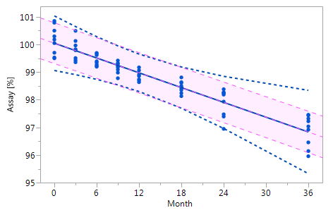 Figure_3_IVFigure_3_IV Figure_3_IVFigure_3_IV |
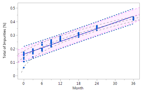 Figure_3_VaFigure_3_Va Figure_3_VaFigure_3_Va |
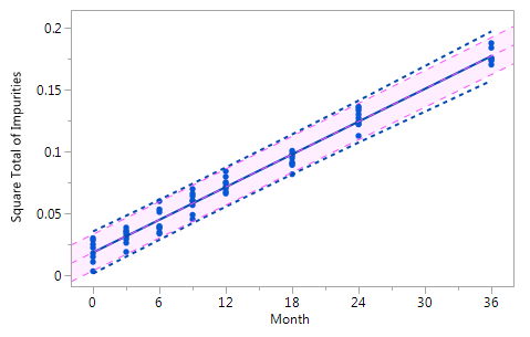 Figure_3_VbFigure_3_Vb Figure_3_VbFigure_3_Vb |
Figure 3 Comparison of the RCR model intervals and the basic linear regression model intervals in different situations
The RCR model fit is represented by the blue solid regression line and the blue dotted lines of the corresponding tolerance interval (95% confidence and 95% coverage). The basic model fit is represented by the purple dashed regression line and the purple shade of the corresponding prediction interval (95% confidence), i.e. the confidence limits for an individual predicted value. The grey dashed lines in panel Va represent the non-linear fit calculated on the basis of the squared response. The six panels compare the RCR model intervals and the basic linear regression model intervals in the following situations: Panel I: "no intercept variation, no slope variation" case; Panel II: "intercept variation, no slope variation" case; Panel III: "no intercept variation, slope variation" case; Panel IV: "intercept variation, slope variation" case; Panel Va: "non-linearity" case; Panel Vb: "non-linearity" case after transformation, i.e. squaring, of the response variable.
Conclusion
The JMP script presented in this manuscript is a suitable and robust tool for assessing stability data of a current batch of a drug product with respect to OOE and OOT results. A prerequisite is the availability of historical stability data of at least three batches with at least four time points of each of these batch.
Bibliography
Carter, R.L, and Yang, M.C.K. Large sample inference in random coefficient regression models. Communications in Statistics – Theory and Methods (1986) 15(8): 2507-2525. LINK
Conover, W.J. (1980), Practical Nonparametric Statistics, New York: John Wiley and Sons, Inc.
ICH Guidance Q1A(R2), Stability Testing of New Drug Substances and Product, step 4 version, 6 February 2003. LINK
Mandel, B.J. Regression Control Chart. J Qual Technol (1969) 1(1): 1-9. LINK
Scholz, F., and Vangel, M. Tolerance bounds and Cpk confidence bounds under batch effects. Published in: Advanced in Stochastic Models for Reliability, Quality and Safety. Edited by Kahle, W., von Collani, E., Franz, J., and Jensen, U. Birkhäuser, Boston, 1998, 361-379. LINK
Shewhart, W.A. (1939). Statistical method from the viewpoint of quality control. (Deming, W.E.). Washington, D.C., The Graduate School, the Department of Agriculture.
Standard Operating Procedure – Laboratory Data Management Guidance – Out of Expectation (OOE) and Out of Trend (OOT) Results. European Compliance Academy (ECA) Analytical Quality Control Working Group, Christopher Burgess, Draft V 0.3, 2015.
United Kingdom Medicines and Healthcare Products Regulatory Agency (MHRA), Out Of Specification Investigations, presentation notes and delegate pack, 28 August 2013. LINK
WHO technical report series, No. 953, Annex 2 Stability testing of active pharmaceutical ingredients and finished pharmaceutical products, 2009. LINK
Presenter
Files
- JMP Discovery Summit Europe 2017 Paper PIDA Tillotts Pharma.docx
- JMP DSE 2017 Regression Control Chart Presentation by PIDA Tillotts Pharma.pptx
- TP_RCC_Script_mod_v3.jsl
- ECA_OOT_Data_Simulation_Case_1.jmp
- ECA_OOT_Data_Simulation_Case_2.jmp
- ECA_OOT_Data_Simulation_Case_3.jmp
- ECA_OOT_Data_Simulation_Case_4.jmp
- ECA_OOT_Data_Simulation_Case_5.jmp
- ECA_OOT_RCC-RCR_Example.jmp
