Linear Mixed Models with JMP® Pro: One Face, Many Flavours*
Jian Cao, PhD
SAS Institute, Inc.
March 24, 2015
Brussels, Belgium
Abstract
One of the new features introduced in JMP Pro 11 is mixed models. This new modelling personality in the Fit Model platform enables one to fit a variety of regression models with fixed and random effects along with an appropriate covariance structure. What’s a mixed model? When and why should one fit a mixed model? And how does JMP fit such a model? In this paper I will try to dispel myths about the mixed models by 1) briefly reviewing the statistical background, 2) discussing why mixed models provide better estimates and consequences of fitting traditional regression models to data where measurements of a response variable are correlated or a key explanatory variable is missing, and 3) illustrating JMP® Pro’s mixed models by fitting different flavours of mixed models that are widely employed in real life applications.
Acknowledgement: I would like to thank Christopher Gotwalt and Laura Lancaster for their help.
*The material presented in this Paper applies to JMP Pro 12 as well. The key enhancement in the new JMP Pro 12 is improved optimization algorithm that enables JMP to run faster than in JMP Pro 11 for large data.
JMP Pro 11 has added a new modeling personality, Mixed Model, to its Fit Model platform. What’s a mixed model? How does JMP fit such a model? What are the key applications where mixed models can be applied? In this paper, I will try to dispel myths about the mixed models and demonstrate JMP’s capability with real-life examples.
What’s a Linear Mixed Model
Linear mixed models are a generalization of linear regression models, y=Xβ+ε. Extending the model to allow for random effects, Z, the new model becomes y=Xβ+Zγ+ε. This is the linear mixed model as there are both fixed effects, X, and random effects, Z.
The following assumptions are made for the random effect parameters, γ and random error ε:
(1) γ and ε are normally distributed, and (2) there are no correlations between and ε. JMP provides several commonly used structures for ε. The fixed effect coefficients, , and covariance matrices for and are jointly estimated by the restricted maximum likelihood method. Fitting mixed models requires additional data on each cross-section unit or, in case of modeling spatial data, dimensions of measurements. There are mixed models for non-normal distributed responses or non-linear mixed models; however, I limit the scope of my discussion to the linear mixed models that are supported in JMP Pro.
Why Mixed Models
When there exists correlation among responses or an important explanatory variable is missing, failure to account for that leads to biased estimates of the effects of treatment and other factors.
Here are some common use cases for mixed models:
- Allowing coefficients
- Analysis of randomized block designs, and split-plot designs where hard-to-change and easy-to-change factors result in multiple error terms;
- Controlling for unobserved individual heterogeneity in the form of random effects (i.e., panel data models);
- Analysis of repeated measures where within-subject errors are correlated;
- Multiple responses that are correlated because measures are taken from the same subjects;
- Subjects are hierarchical (i.e., students within schools). This is known as Hierarch Linear Model or Multi-level Models;
- Spatial variability (i.e., geospatial regression);
With JMP Pro you can easily specify and fit all of these models using the point-and-click interface and review the results in a user-friendly way.
Steps to Specify a Mixed Model in JMP Pro
- 1. Select Analyze =>Fit Model, and choose Mixed Model Personality;
- 2. Select a continuous response variable from you data table as Y and construct fixed effects as you normally would do with a standard least squares fit;
3A. Use Random Effects tab to specify random coefficients or random effects;
3B. Use Repeated Structure tab to select a covariance structure for model errors;
- 4. Click Run.
I’ll now turn to example to show four different flavours of mixed models: random coefficient model, analysis of repeated measures, panel data model and geospatial regression.
Example 1: Random Coefficient Models—allowing intercept and slopes to vary randomly across subjects
In this example we are interested in estimating the effect on wheat yield of pre-planting moisture in the soil while allowing each wheat variety to have random deviation from population effects. So, a random coefficient model is called for. The experiment randomly selects 10 varieties from wheat population and assigns each to six plots of land. In total, 60 observations with 6 measurements of yield for each variety is collected. (The data, “Wheat”, is available in JMP’s Sample Data directory.)
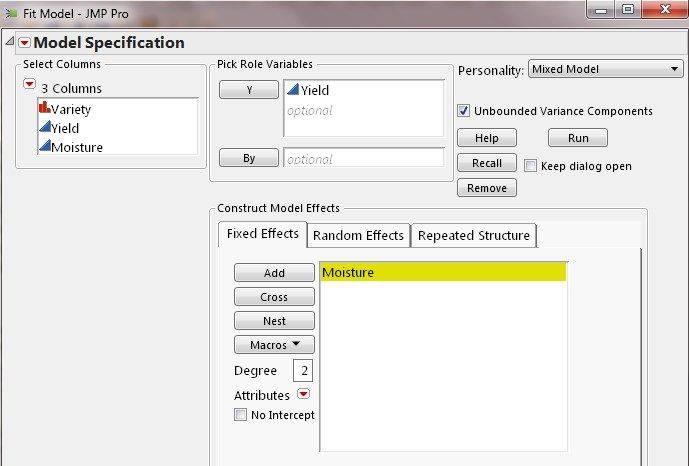
I followed the steps laid out above to specify the model. From Fixed Effects tab, specify Moisture along with a default intercept as fixed effects.
Next, from the Random Efects tab,using Nest Random Coefficients button to request random intercept and Moisture effect for each variety. 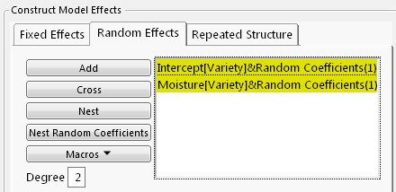
Lastly, from Repeated Structure tab, select Residual for the model error term.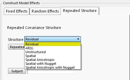
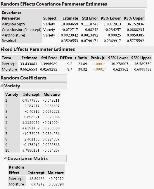
The following screenshot shows Random Effects Covariance Parameter Estimates, Fixed Effects Parameter Estimates and Random Coefficients. Let’s discuss them in turn.
The variance estimate for Intercept is 18.89 with a standard error estimate of 9.11, so the z-score is 2.07 (=18.89/9.11). Using the Normal Distribution function from JMP Formula Editor we can find the p-value to be 0.0192, indicating that the variation in baseline yield across varieties is statistically significant. Similarly, the p-value for Cov(Moisture, Intercept), 0.3777, and p-value for Var(Moisture) is 0.0380.
The Random Coefficients report gives the BLUP (Best Linear Unbiased Predictor) values for how each variety is different from the population intercept and population Moisture effect reported in Fixed Effects Parameter Estimates. For Variety 1, the estimated moisture effect on its yield is 0.61 (=0.66-0.05), and baseline yield is 34.39 (=33.43+0.96) and the predicted yield equation is
Combining both the fixed effects and random coefficient estimates, we find a significant overall effect on wheat yield of moisture, and discover significant variation in the moisture effect across different varieties.
Other Applications of Random Coefficient Models
Individual Growth Model is a type of random coefficient model in which random time effect is estimated for each individual. His is done by specifying a continuous time variable such as day or month as a random effect, and using Nest Random Coefficients button to request separate slope (i.e., growth) and intercept for each individual.
In educational research, subjects are often nested in a hierarchical order. By adding multiple groups of random effect statements you can fit Hierarchical Linear Models/Multi-level Models.
Example 2: Analysis of Repeated Measures—accounting for correlated errors
Repeated measures are the multiple measurements of a response collected from the same subjects over time. In this clinical trial, subjects (i.e., patients) were randomly assigned to different treatment groups. Each subject’s total cholesterol level was measured several times during the trial. The objective of the study is to test whether new drugs are effective at lowering cholesterol. What makes the analysis of repeated measures distinct is the correlation of the measurements within a subject. Failure to account for it often leads to incorrect conclusion about the treatment effect. (The data, Cholesterol Stacked, is available in JMP’s Sample Data directory.
JMP Pro offers three commonly used covariance structures:
- Unstructured
- AR(1) (first-order autoregressive) estimates correlation between two measurements that are one unit of time apart. The correlation declines as the time difference increases.
- CS
The following screenshot shows the Fixed Effects part of the repeated measures analysis, which includes Treatment, Month, AM/PM, and their interactions.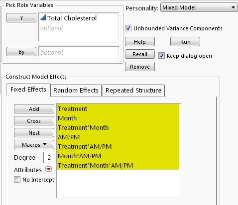
I will consider three different covariance structures for the within-subject errors. First, let’s use Unstructured. Apply Time column as Repeated, and Patient column as Subject--this defines the repeated measurements within a subject. It is important to note that JMP requires that Subject column be uniquely valued and that Repeated column be categorical for the Unstructured option.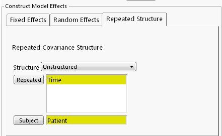
Key reports include Repeated Effects Covariance Parameter Estimates, Fixed Effects Parameter estimates, and Tests Fixed Effects Tests.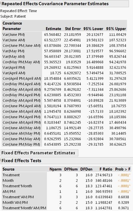
One way of testing statistical significance of the covariance estimates is to calculate the z-scores and find their p-values, as I did in the previous random coefficient model example. However, we can check the confidence limits: if the 95% confidence interval for a covariance estimate includes zero, then we can say that the estimate is not statistically significant from zero at α=5%. As we can see, all six variance estimates are significantly different from zero but most of covariance estimates are not. This suggests that a parsimonious structures, such as AR (1), should be considered.
Fixed Effects Tests report shows a highly significant treatment effect. Cholesterol level is also found to vary significantly from month to month and from morning to afternoon.
Next, we consider AR(1) as the covariance structure for the within-subject errors. Please note that Repeated column used in AR(1) by JMP must be a continuous variable. So, Days—number of days from the trial start date at each measurement--is used instead of a categorical variable used for the UN option.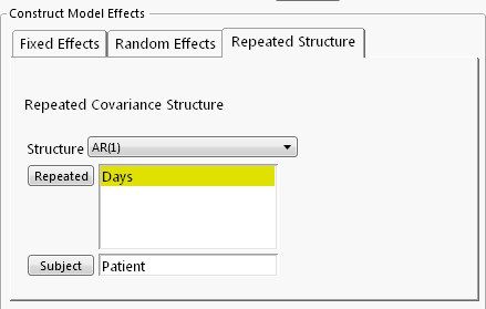
The Repeated Effects Covariance Parameter Estimate report shows a highly significant within-subject correlation of 0.95. Fixed effects results are similar to those in the UN option (not shown)--treatment effect and time effects are statistically significant.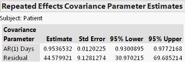
To complete our example, finally, let’s fit the model with a CS structure. To do so, select Residual as the Repeated Covariance Structure—but no need to specify Repeated and Subject columns with this option; instead, we add the subject ID, Patient, as a random effect on the Random Effects tab. That is
within-subject covariance is modelled through the subject effect.

Judged by the 95% confidence limits, the covariance between any two measures on the same subject is not statistically significant at α=0.05 (actually, p-value= 0.0621). Fixed effect test results are similar to the previous models and are thus not shown here.
So, which repeated structure should be adopted? One criterion for model comparison is AICc. From the Fit Statistics reported by JMP (not shown), AICcs are: Unstructured—703.84, AR(1)—652.63 and CS—832.55. So, AR(1) is the winner.
Example 3: Panel Data Models--controlling for unobserved heterogeneity
This example is taken from Vella and Verbeek (1998), which is discussed in Introductory Econometrics by Jeffrey Woodridge as Example 14.4. See references below for more info.
The original data came from the National Longitudinal Survey of Youth 1979 Cohort (NLSY79). In the data, each of the 545 male workers worked every year from 1980 through 1987. We’re interested in estimating the effect on wage earnings of union membership controlling for education, work experience, ethnicity, etc.
Although NLSY79 collects detailed background information on the workers to be used as control variables, there is still individual difference that cannot be observed or measured. Panel data provides a way of accounting for individual heterogeneity: if the unobserved heterogeneity can be assumed to be uncorrelated with all the explanatory variables included in the model, we can account for it by treating it as a random effect.
Following Woodridge’s discussion a Log(Wage) equation is fit in which worker’s ID is entered as a random effect to capture the unobserved differences.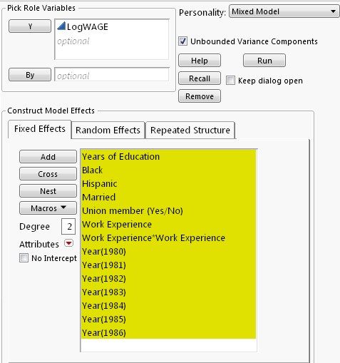
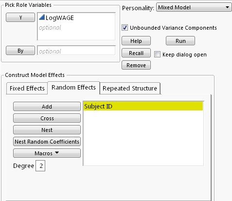
I select Residual for the mode error term. The model is called one-way random effect model in econometrics.
The results are shown below.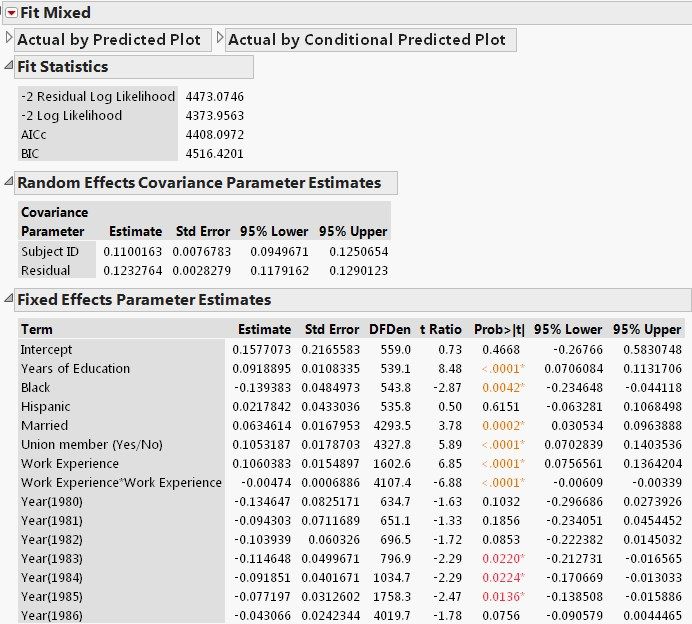
From the Random Effects Covariance Parameter Estimates report we find that individual heterogeneity accounts for 47.8% (=0.11/(0.11+0.12)) of the total variation, indicating a large unobserved heterogeneity effect. In other words, an OLS analysis would likely yield misleading results.
The Fixed Effects Parameter Estimates report shows an estimated rate of return to education at 9.2% and a union premium of 10.5%, both of which are highly statistically significant. As a comparison, a pooled OLS would estimate the union premium at 18.2%. See Woodridge (2013, Page 495).
References
Francis Vella and Marno Verbeek (1998), "Whose Wages Do Unions Raise? A Dynamic Model of Unionism and Wage Rate Determination for Young Men", Journal of Applied Econometrics, Vol. 13, No. 2, pp. 163-183. Data can be downloaded from Journal’s website http://qed.econ.queensu.ca/jae/1998-v13.2/vella-verbeek/
Jeffrey M. Woodridge (2013), Introductory Econometrics: A Modern Approach (5th ed), CENGAGE Learning.
Example 4: Modeling geospatial data--taking spatial correlation into account
Like repeated measures are correlated over time, spatial data are likely correlated in space. That is, measurements that are relatively close together are more alike than those farther apart. Thus, we need to take spatial dependency into account in the analysis.
Spatial data are recorded along with coordinates such as latitude and longitude, positions of row and column, north-south and east-west directions. The distance between two measurements are calculated using a Euclidean distance function, which is used to form a covariance structure. If a distance function doesn’t depend on the directions of measurements, then the covariance is said to be isotropic; otherwise it is anisotropic. In addition, a nugget effect can be added to account for abrupt changes over small distances in a local area.
JMP Pro provides four Euclidean distance functions for isotropic structures: power, exponential, Gaussian and spherical. Various forms of anisotropic structures are available. A nugget effect can also be added to covariance structures.
The following example is taken from SAS for Mixed Models, 2nd Edition, 2006, pp. 457-460. (http://www.sas.com/store/prodBK_59882_en.htm). In order to investigate the water drainage at a hazardous waste disposal site, 30 samples were taken at various locations at the site and recorded by their north-south and east-west directions. A linear relationship between water drainage (measured by log-transmissivity) and the thickness of a layer of salt was proposed. (The data, Hazardous Waste, is Data Set 11.6 in the zipped file
http://support.sas.com/publishing/bbu/59882/59882.zip.)
A spatial regression model is fit using a spatial anisotropic power structure with a nugget effect. This structure allows (1) distance to be a power function of spatial correlation, (2) spatial correlations to differ in different directions, and (3) variation over small distances.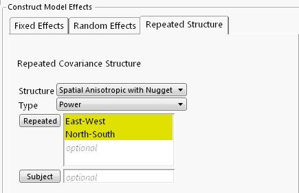
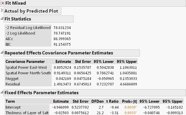
Covariance Parameter Estimate report suggests highly significant spatial correlation and that two correlation coefficients are, respectively, 0.81 (East-West) and 0.91 (North-South). However, there appears to have no nugget based on the confidence limits. Fixed Effects Parameter Estimates show a significant negative effect (-0.025) on water drainage of thickness of salt.
I refit the model by removing the nugget effect.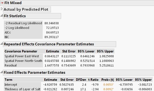
We notice some minor changes: the estimated spatial correlations are 0.86 and 0.82, respectively, and effect of thickness of salt is -0.021. Comparing the goodness of fit using AICc, the second model is slightly better as its AICs is smaller (84.7 vs. 86.4)
To formally test the existence of spatial correlation, we fit an independent errors model by selecting Residual as the structure (i.e. assuming no spatial correlation). The difference in -2 Residual Log Likelihood value between the two models forms a χ2 likelihood ratio test. The -2 Residual Log Likelihood from the independent errors model is 94.07, so the difference is a 13.72 (=94.07-80.35). This yields a p-value of 0.001 for DF=2. Therefore, significant spatial correlation is found at this site.
Summary
Hopefully, these examples have illustrated the versatility of linear mixed models and ease of fitting a mixed model with JMP. Before I close I’d like to share some general tips.
- In order to run a mixed model, data needs to be organized in a “tall & skinny” format where multiple measures of a response are stacked into a single column. If your data is in a “short & wide” format, use the JMP Tables function Stack to transpose.
- Follow the JMP Repeated Covariance Structure Requirements when entering Repeated and Subject columns. http://www.jmp.com/support/help/Launch_the_Mixed_Model_Personality.shtml#1013652
- Try different covariance structures and evaluate different models by comparing AICc or BIC. The smaller the AICc (or BIC), the better fit of a model. Ceteris paribus, a parsimonious model is better.
- An independent errors model (i.e. a model with only fixed effects) can serve as a baseline model to perform a χ2 likelihood ratio test on the existence of a covariance e structure.
- Keep in mind that when both random effects and repeated effects are included in a model there is often insufficient data to estimate both effects.
