Step Stress Modeling in JMP using R (2020-US-30MP-574)

[#1]

Level: Intermediate

Charles Whitman, Reliability Engineer, Qorvo

Simulated step stress data where both temperature and power are varied are analyzed in JMP and R. The simulation mimics actual life test methods used in stressing SAW and BAW filters. In an actual life test, the power delivered to a filter is stepped up over time until failure (or censoring) occurs at a fixed ambient temperature. The failure times are fitted to a combined Arrhenius/power law model similar to Black’s equation. Although stepping power simultaneously increases the device temperature, the algorithm in R is able to separate these two effects. JMP is used to generate random lognormal failure times for different step stress patterns. R is called from within JMP to perform maximum likelihood estimation and find bootstrap confidence intervals on the model estimates. JMP is used live to plot the step patterns and demonstrate good agreement between the estimates and confidence bounds to the known true values.  A safe-operating-area (SOA) is generated from the parameter estimates.  The presentation will be given using a JMP journal.

The following are excerpts from the presentation.

Auto-generated transcript...

Speaker	Transcript
CWhitman	All right. Well, thank you very much for attending my talk. My name is Charlie Whitman. I'm at Corvo and today I'm going to talk about steps stress modeling in JMP using R.
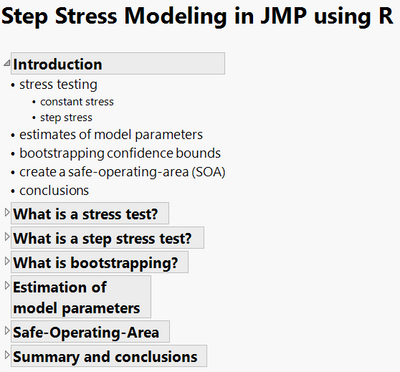
	So first, let me start off with an introduction. I'm going to talk a little bit about stress testing and what it is and why we do it.
	There are two basic kinds. There's constant stress and step stress; talk a little bit about each. Then when we get out of the results from the step stress or constant stress test
	are estimates of the model parameters. That's what we need to make predictions. So in the stress testing, we're stressing parts of very high stress and then going to take that data and extrapolate to use conditions, and we need model parameters to do that.
	But model parameters are only half the story. We also have to acknowledge that there's some uncertainty in those estimates and we're going to do that with confidence bounds and I'm gonna talk about a bootstrapping method I used to do that.
	And at the end of the day,
	armed with our maximum likelihood estimates and our bootstrap confidence bounds, we can create something called the safe operating area,
	SOA, which is something of a reliability map. You can also think of it as a response surface. So we're going to get is...find regions where it's safe to operate your part and regions where it's not safe. And then I'll reach some conclusions.
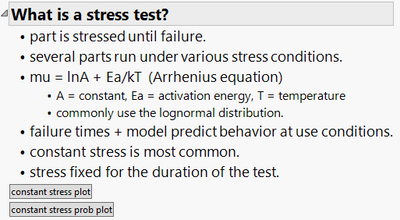
	So what is a stress test? In a stress test you stress parts until failure. Now sometimes you don't get failure; sometimes parts, you have to start, stop the test and do something else.
	And that case, you have a sensor data point, but the method of maximum likelihood, which are used in the simulations takes sensoring into account so you don't have to have 100% failure. We can afford to have some parts not fail.
	So what you, what you do is you stress these parts under various conditions, according to some designed experiment or some matrix or something like that. So you might run
	your stress might be temperature or power or voltage or something like that and you'll run your parts under various conditions, various stresses and then take those that data fitted to your model and then extrapolate to use conditions.
	mu = InA + ea/kT.
	Mu is the log mean of your distribution; we commonly use the lognormal distribution. That's going to be a constant term plus the temperature term.
	You can see that mu is inversely related to temperature. So as temperature goes up, mu goes down, and that's temperature goes down, mu goes up. If we can use the lognormal, you will also have an additional parameter that the shape factor sigma.
	So after we run our test, we will run several parts under very stressed conditions and we fit them to our model. It's then when you combine those two that you can predict behavior at use conditions, which is really the name of the game.
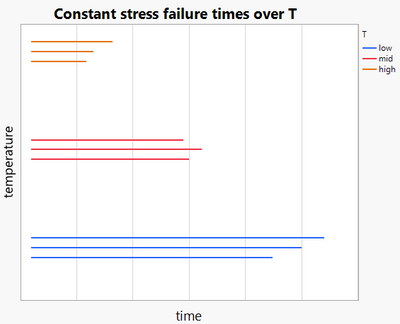
	The most common method is a is a constant stress test, and what basically, the stress is fixed for the duration of the test. So this is just showing an example of that. We have a plot here of temperature versus time.
	If we have a very low temperature, say you could get failures that would last time...that sometimes be very long.
	The failure times can be random, again according to, say, some distribution like the lognormal. If we increase the temperature to some higher level,
	we would get end of the distribution of failure times, but on the average the failure times would be shorter.
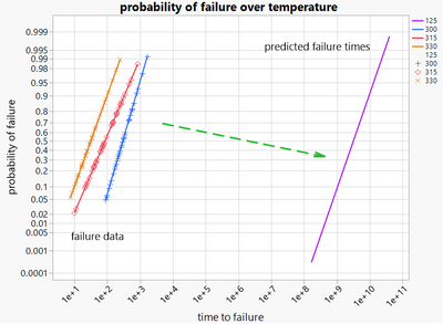
	And if we increase the temperature even more, same kind of thing, but failure times are even shorter than that. So what I can do is if I ran, say, a bunch of parts under these different temperatures, I could fit the results to a probability plot that looks like this.
	I have probability versus time to failure at the highest temperature here. This example is 330 degrees C, I have my set of failure times which I set to lognormal. And then as I decrease the temperature lower and lower the failure times get longer and longer.
	Then I take all this data over temperature I fit it to the Arrhenius model, I extrapolate. And then I see I can get my predictions at use conditions. This is what we are after.
	I want to point out that when we're doing these accelerated testing, this test, we have to run at very high stress because, for example,
	even though this is, say, lasting 1000 hours or so, our predictions are that the part under use conditions would be a billion hours and there's no way that we could
	run test for a billion hours. So we have to get tests done in a reasonable amount of time and that's why we're doing accelerated testing.
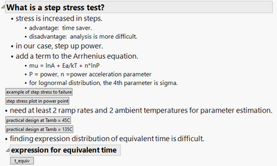
	So then, what is a step stress? Well, as you might imagine, a step stresses where you increase the stress in steps
	or some sort of a ramp. The advantage is that it's a real time saver. As I showed in the previous plot,
	those tests could last a very long time that could be 1000 hours. So that's it could be weeks or months before the test is over. A step stress test
	could be much shorter or you might be able to get done in hours or days. So it's a real time saver. But the analysis is more difficult and I'll show that in a minute.
	So, in the work we've done at Corvo, we're doing reliability of acoustic filters and those are those are RF devices. And so the stress in RF is RF power.
	And so we step up power until failure.
	So if we're going to step up power, we can do is we can model this with this expression here. Basically, we had the same thing as the Arrhenius equation, but we're adding another term, n log p.
	N is our power acceleration parameter; p is our power. So for the lognormal distribution, there would be a fourth parameter, sigma, which is the shape factors. So you have 1, 2, 3, 4 parameters.
	Let me just give you a quick example of what this would look like.
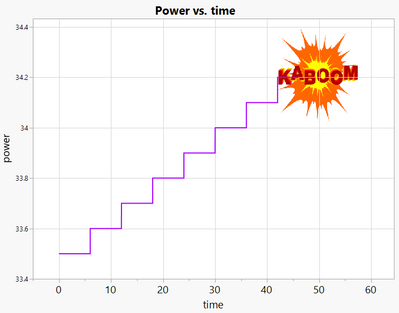
	You start, this is power versus time. Power is in dBm. You're starting off at some power like 33.5 dBm, you step and step and step and step until hopefully you get failure.
	And I want to point out that
	your varying power, and as you increase the power to the part, that's going to be changing the temperature. So as power is ramped, so it is temperature. So power and temperature are then confounded.
	So you're gonna have to do your experiment in such a way that you can separate the effects of temperature and power. So I want to point out that
	you have these two terms (temperature and power), so it's not just that I increase the power to the part and it gets hotter and it's the temperature that's driving it. It's power in and of itself also increases the failure rate.
	Right. So now if I show a little bit more detail about that step stress plot.
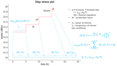
	So here again a power versus time. I'm running a part for, say, five hours at some power, then I increase the stress, and run another five hours, and increase the stress on up until like a failure.
	So, and as I mentioned as the power is increasing, so is the temperature. So I have to take that into account somehow. I have to know what the
	t = T ambient + R th times p
	T ambient is our ambient temperature; P is the power; and R th is called the thermal impedance which is a constant. So, that means, as I set the power, so I know what the power is and then I can also estimate what the temperature is for each step.
	So what we'd like to do is then take somehow these failure times that get from our step stress pattern and extrapolate that to use conditions.
	If I was only running, like, for time delta t here only
	and I wanted to extrapolate that to use conditions, what I would do is I would multiply...get the equivalent amount of time delta t times the acceleration factor. And here's the acceleration factor. I have an activation energy term, temperature term, and a power term.
	And so what I would do is I would multiply by AF. And since I'm going from high stress down to low stress, AF is larger than one and this is just for purposes of illustration, it's not that much bigger than one, but you get the idea.
	And as I increase the power, temperature and power are changing so the AF changes with each step.
	So if I want to then get the equivalent time at use conditions, I'd have to do a sum. So I have each segment.
	It has its own acceleration factor and maybe its own delta t. And then I do a sum and that gives me the equivalent time.
	So this, this expression that I would use them to predict equipment time if I knew exactly what Ea was and exactly what n was, I could predict what the equivalent time was. So that's the idea.
	So it turns out that....so as I said, temperature and power are confounded. So in order to estimate, what we do is we have to run to two different ambient temperatures
	If you have the ambient temperatures separated enough, then you can actually separate the effects of power and temperature.
	You also need at least two ramp rates. So at a minimum, you would need a two by two matrix of ramp rate and ambiant temperature.
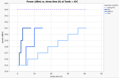
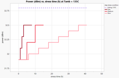
	In the simulations I did, I chose three different rates as shown here. I have power in dBm versus stress time
	And I have three different ramps, but with different rates. I'll have a fast, a medium, and a slow ramp rate. In practice, you would let this go on and on and on until failure, but I've only just arbitrarily cut it off after a few hours. You see here also I have a ceiling.
	The ceiling is four; it's because we have found that if we increase the stress or power arbitrarily, we can change the failure mechanism.
	And what you want to do is make sure that failure mechanism, when you're under accelerate conditions is the same as it is under use conditions. And if I change the
	failure mechanism that I can't do an extrapolation. The extrapolation wouldn't be valid.
	So we had the ceiling here of drawn to 34.4 dBm, and we even given ourselves a little buffer to make sure we don't get close to that.
	So our ambient temperature is 45 degrees C, we're starting it a power 33.5 dBm so we would also have another set of conditions at
	135 degrees. See, you can see the patterns here are the same. And we have a ceiling and they have a buffer region, everything, except we are starting at a lower power. So here we're below 32 dBm, whereas before we were over 33.
	And the reason we do that is because if we don't lower the power at this higher temperature, what will happen is you'll get failures almost immediately if you're not careful, and then you can't use the data to do your extrapolation.
	Alright, so what we need, again, is an expression for our quivalent time, as I showed that before. Here's that expression. This is
	kind of nasty and I would not know how to derive from first principles of what the expression is for the distribution of the equivalent time of use conditions. So, when faced with something which is kind of difficult like that, what I choose to do was use the bootstrap.
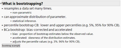
	So what is bootstrapping?
	So with bootstrapping, what we're doing is we are resampling the data set many times with replacement. That means from the original data set of observations, you can have replicates of from the original data set or maybe an observation won't appear all.
	And the approach I use is called non parametric, because we're not assuming the distribution. We don't have to know the underlying distribution of the data.
	So when you generate these many bootstrap samples, which you can get as an approximate distribution of the parameter, and that allows you to do statistical inference. In particular, we're interested in putting in confidence bounds on things. So that's what we need to do.
	Simple example of bootstrapping is called percentile bootstrap. So, for example, suppose I wanted 90% confidence bounds on some estimate.
	And I would do is I would form, many, many bootstrap replicates and I would extract the parameter from each bootstrap sample. And then I would sort that and I would figure out which is the shift and 95th percentile from that vector and those would form my 90% confidence bounds.
	What I did actually in my work was I used an improvement over to percentile, a technique. It's called the BCa for bias corrected and accelerated.
	Bias because sometimes our estimates are biased and this method would take that into account.
	Accelerated, unfortunately the term accelerated is confusing here. It has nothing to do with accelerated testing, it has to do with the method, the method has to do for with adjusting
	for the skewness of the distribution. But ultimately you're...what you're going to get is
	it's going to pick for you different percentile values. So, again, for the percentile technique we had fifth and 95th.
	The bootstrap or the BCa bootstrap might give you something different, might say the third percentile and 96% or whatever. And those are the ones who would need to choose for your 90% confidence bounds.
	So I just want to run through a very quick example just to make this clear.
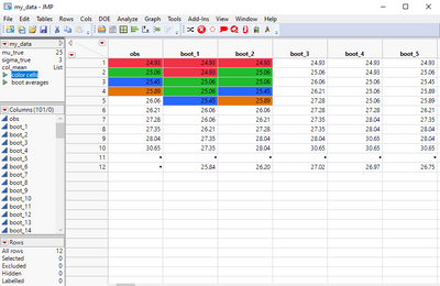
	Suppose I have 10 observations and I want to do for bootstrap samples from this, looking something like this. So, for example, the first observation here 24.93 occurs twice in the first sample, once in the second sample, etc.
	25.06 occurs twice. 25.89 does not occur at all and I can do this, in this case, 100 times
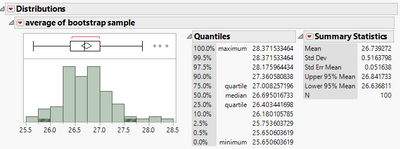
	And for each bootstrap sample then, I'm going to find, in this case I'm gonna take the average, say, I'm interested in the distribution of the average. Well, here I have my distribution of averages.
	And I can look to see what that looks like. Here we are.
	It looks pretty bell shaped and I have a couple points here, highlighted and these would be my 90% confidence bounds if I was using the percentile technique.
	So here's this is the sorted vector and the fifth percentile is at 25.84 and the 95th percentile is 27.68.
	If I wanted to do the BCa method, I would might just get some sort of different percentile. So this case, 25.78 and 27.73. So that's
	very quickly, what the BCa method is. So in our case, we'd have samples of...
	we would do bootstrap on the stress patterns. You would have multiple samples which would have been run, simulated under those different stress patterns and then
	bootstrap off those. And so we're going to get a distribution of our previous estimates or previous parameters, logA, EA, and sigma
	Right.
CWhitman	So again, here's our equation.
	So again, JMP
	The version of JMP that I have does not do bootstrapping. JMP Pro does, but the version I have does not, but fortunately R does do bootstrapping. And I can call R from within JMP. That's why I chose to do it this way. So I have
	I can but R do all the hard work. So I want to show
	an example, what I did was I chose some known true values for logA, EA and sigma. I chose them over some range randomly.
	And I would then choose that choose the same values for these parameters of a few times and generate samples each time I did that. So for example, I chose minus 28.7 three times for logA true and
	we get the data from this. There were a total of five parts per test level or six test levels, if you remember, three ramps, two different temperatures, six levels, six times five is 30.
	So there were 30 parts total run for this test and looking at the logA hat, the maximum likelihood estimates are around 28 or so.
	So that actually worked pretty well. I can look at...now for my next sample, I did three replicates here, for example, minus 5.7 and how did it look when I ran my method of the maximum that are around that minus 5.7 or so. So the method appears to be working pretty well.
	But let's do this a little bit more detail.
	Here I ran
	the simulation a total of 250 times with five times for each group.
	LogA true, EA true are repeated five times and I'm getting different estimates for logA hat, EA, etc.
	I'm also putting...using BCa method to form confidence bounds on each of these parameters, along with the median time to failure. So let's look and just plot this data to see how well it did.
	You have logA hat versus logA true here and we see that the slope is about right around 1 and the intercept is not significantly different than 0, So this is actually doing a pretty good job. If my logA true is
	at minus 15 then I'm getting right around minus 15 plus or minus something for my estimate. And the same is true for the other parameters EA, n and sigma, and I even did my at a particular p zero P zero. So this is all behaving very well.
	We also want to know, well how well is the BCa method working? Well, turns out, it worked pretty well.
	I want to...the question is how successful was the BCa method. And here I have a distribution. Every time I correctly correctly bracketed the known true value, I got a 1. And if I missed it, I got a 0.
	So for logA I'm correctly bracketing the known true value 91% of the time. I was choosing 95% of the time, so I'm pretty close. I'm in the low 90s and I'm getting about the same thing for activation, energy and etc. They're all in the mid to low 90s. So that's actually pretty good agreement.
	Let's suppose now I wanted to see what would happen if I increase the number of bootstrap iterations and boot from 100 to 500. What does that look like?
	If I plot my MLE versus the true value, you're getting about the same thing.
	The estimates are pretty good. The slope is all always around 1 and the intercept is always around 0. So that's pretty well behaved.
	And then if I look at the confidence bound width,
	See, on the average, I'm getting something around 23 here for confidence bound width, and around 20 or so for mu and getting something around eight for
	value n. And so these confidence bands are actually somewhat wide.
	And I want to see what happens. Well, suppose I increase my sample size to 50
	instead of just using five? 50 is not a realistic sample size, we could never run that many. That would be very difficult to do, very time consuming.
	But this is simulation, so I can run as many parts as I want. And so just to check, I see again that the maximum likelihood estimates agree pretty well with the known true values. Again, getting a slope of 1 and intercept around zero.
	And BCa,
	I am getting bracketing right around 95% of the time as expected. So that's pretty well behaved too and my confidence bound width,
	now it's much lower. So, by increasing the sample size, as you might expect, the conference bounds get correspondingly lower.
	This was in the upper 20s originally, now it's around seven. This is also...the mu was also in the upper 20s, this is now around five; n was around 10 initially, now it's around 2.3, so we're getting this better behavior by increasing our sample size.
	So this just shows what the summary, this would look like.
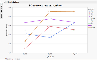
	So here I have a success rate versus these different groups; n is the number of parts per test level.
	And boot is the number of bootstrap samples I created. So 5_100, 5_500 and 50_500 and you can see actually this is reasonably flat. You're not getting
	big improvement in the coverage. We're getting something in the low to mid 90s, or so. And that's about what you would expect.
	So by changing the number of bootstrap replicates or by changing the sample size, I'm not changing that very much. BCa is equal to doing a pretty good job, even with five parts per test level and 100 bootstrap iterations.
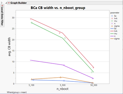
	About the width.
	But here we are seeing a benefit. So the width of the confidence bounds is going down as we increase the number of bootstrap iterations. And then on top of that,
	if you increase the sample size, you get a big decrease in the confidence bound width. So all this behavior is expected,
	but the point here is, this simulation allows you to do is to know ahead of time, well, how big should my sample size be?
	Can I get away with three parts per condition? Do I need to run five or 10 parts per condition in order to get the width of the confidence bounds that I want?
	Similarly, when I'm doing analysis, well, how many bootstrap iterations do I have to do to kind of get away with 110? Do I need 1000? This also gives you some heads up of what you're going to need to do when you do the analysis.
	Alright, so finally, we are now armed with our maximum likelihood estimates and our confidence bounds. So we can do
	We can summarize our results using the safe operating area and, again
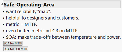
	what we're getting here is something of a reliability map or a response surface of temperature versus power. So you'll have an idea of how reliable the part is under various conditions.
	And this can be very helpful to designers or customers. Designers want to know when they create a part, mimic a part, is it going to last?
	Are they designing a part to run at to higher temperature or to higher power so that the median time to failure would be too low.
	Also customers want to know when they run this part, how long is the part going to last? And so what the SOA gives you is that information.
	The metric I'm going to give here is median time to failure. You could use other metrics. You could use the fit rate you could use a ???, but for purposes of illustration, I'm just using median time to failure.
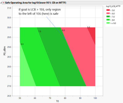
	An even better metric, as I'll show, is a lower confidence bound on the median time to failure. It's a gives you a more conservative estimate
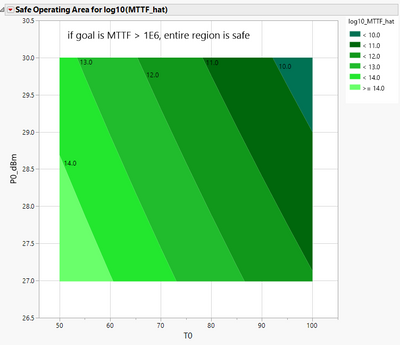
	So ultimately, the SOA then will allow you to make trade offs then between temperature and power. So here is our contour plot showing our SOA.
	These contours are log base 10 of the median time to failure. So we have power versus temperature, as temperature goes down and as power goes down, these contours are getting larger and larger. So as you lower the stress as you might expect, and median time to failure goes up.
	And suppose we have a corporate goal and the corporate goal was, you want the part to last or have a median time to failure greater than 10 to six hours.
	If you look at this map, over the range of power and temperature we have chosen, it looks like we're golden. There's no problems here. Median time to failure is easily 10 to six hours or higher.
	So that tells us we have to realize that median time failure again is an average, an average is only tell half the story. We have to do something that acknowledges the uncertainty in this estimate. So what we do in practice is use a lower conference bound on the median time to failure here.
	So you can see those contours have changed, very much lower because we're using the lower confidence bound, and here, 10 to the six hours is given by this line.
	And you can see that it's only part of the reach now. So over here at green, that's good. Right. You can operate safely here but red is dangerous. It is not safe to run here. This is where the monsters are. You don't want to run your part this hot.
	And also, this allows you to make trade offs. So, for example, suppose a designer wanted to their part to run at 80 degrees C.
	That's fine, as long as they keep the power level below about 29.5 dBm.
	Similarly, suppose they wanted to run the part at 90 degrees C. They can, that's fine as long as they keep the power low enough, let's say 27.5 dBm. Right. So this is where you're allowed to make trade offs for between temperature and power.
	Alright, so now just to summarize.
	So I showed the differences between constant and step stress testing and I showed how we extract extract maximum likelihood estimates and our BCa confidence bounds from the simulated step stress data.
	And I demonstrated that we had pretty good agreement then between the estimates and the known true values. In addition,
	BCa method worked pretty well, even with n boot of only 100 and five parts per test level, we had about 95% coverage.
	And that coverage didn't change very much as we increased the number of bootstrap iterations or increased the sample size. However, we did see a big change on the confidence bounds width.
	And that the results there showed that we could make some sort of a trade off. Again, we could, you know, from the simulation, we would know how many bootstrap iterations do we need to run and how many parts per test conditions we need to run.
	And ultimately, then we took those maximum likelihood estimates and our bootstrap confidence bounds and created the SOA, which provides guidance to customers and designers on how safe a particular T0/P0 combination is.
	And then from that reliability map, then we able to make a trade off between temperature and power.
	And lastly, I showed that using the lower confidence bound on the median time to failure
	does provide a more conservative estimate for the SOA. So, in essence, using the lower confidence bound makes the SOA, the safe operating area, a little safer. So that ends my talk. And thank you very much for your time.