- JMP User Community
- :
- Blogs
- :
- JMP Blog
- :
- Analyzing spectroscopic data: Pre-processing
- Subscribe to RSS Feed
- Mark as New
- Mark as Read
- Bookmark
- Subscribe
- Printer Friendly Page
- Report Inappropriate Content
My colleague Jeremy Ash (@JeremyAshJMP) and I realize that analyzing spectroscopic data has many nuances and potential pitfalls that can make analysis difficult and messy at best. So we wanted to write this blog series to describe how you can import, visualize, clean, and analyze spectroscopic data with JMP software.
To make it easier for you to try out some of these steps on your own data, we have created the Spectral Tools add-in, which you can learn more about and download here in the JMP Community. This is a simple add-in that streamlines some of the data import and visualization methods discussed in this blog post. It is only a prototype, and only a first step toward providing some convenient functions for spectral data. You can give us feedback in the comments of this blog post or on the add-in page.
In this post, we are analyzing a near-infrared data set from Martens et al. "Light Scattering and light absorbance separated by extended multiplicative signal correction. Application to near-infrared transmission analysis of powder mixtures" Analytical Chemistry 2003 Feb1;75(3):394-404. We will show how pre-processing improves the overall quality of the data and allows you to see, in this case, grouping based on proportions of constituents much more clearly.
Importing spectra
When importing spectra, the Spectral Tools add-in assumes that each spectra is in a separate file in a single directory. The spectra can be in delimited text files (.csv or .tsv, for example) or JCAMP-DX files. Only JCAMP-DX without compression is supported. The stacked format is the default data table format in Spectra Tools. You can also import files in wide format. In this blog post, we most frequently use the stacked format, but a few of the pre-processing steps require the wide format. You can convert between the stacked and wide formats using the Stack and Split commands in the Tables menu in JMP.
Data visualization
As with any new data, once you get it into your analytics software of choice, we highly recommend visualizing the state of the data, and regularly comparing to this first look after any pre-processing is done. In JMP, we use the Graph Builder platform to help with the visualization.
Figure 1 shows a line plot of the spectra in Graph Builder. With your data in the stacked format, drag the X and Y variables to their respective axis, and use the spectra ID as the overlay variable. Alternatively, you can use the Launch Graph Builder command in Spectra Tools. For the color variable, we use the response variable of interest, which is gluten content.
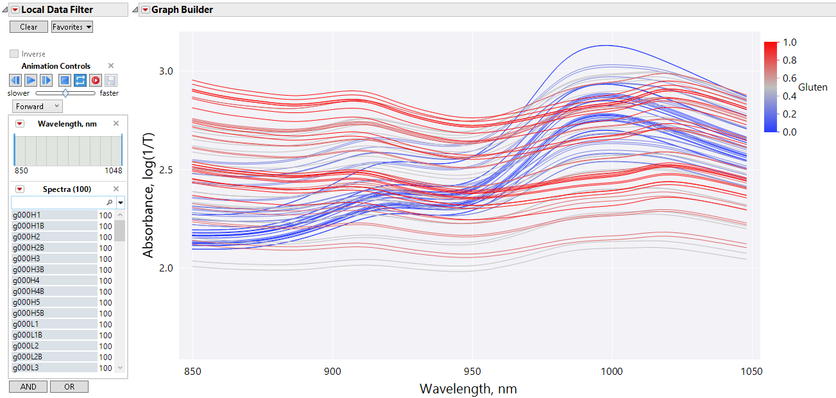
To zoom into regions of interest (ROIs), click and drag the X axis. You can create a Local Data Filter in the red triangle menu for a few other useful controls. This is provided by default in Spectral Tools. These are shown on the left of Figure 1. The wavelength local data filter can be used to focus on a region of interest (ROI). To create a new data table for just the ROI data, go to the local data filter red triangle and select Show Subset. Also, to only show a subset of the spectra on the graph, select the spectra in the spectra ID Local Data Filter. You can also use the Animation Controls to cycle through one spectra at a time.
For more complicated selections like multiple ROIs, you can plot the spectra as points and select the points of interest. The Subset command in the Table menu can be used to create a data table with just the ROI data.
One important thing to remember about Graph Builder is that once you have finished setting up the graph the way you want it, you can save the script to the data table, so that the same plots can be easily recreated with new data. For example, you may wish to recreate your graph when comparing spectra before and after pre-processing. Another option for comparing spectra before and after pre-processing is to use the Launch Graph Builder command in Spectral Tools.
Also, new in JMP 16 in Graph Builder, Savitzky-Golay (SG) smoothing can be applied as an initial pre-processing step (Figure 2). Once you select your tuning parameters, you can output the smoothed data. Go to the smoother red triangle and select Save Formula. Note that this will require your wavelength to be a continuous variable (you can modify the variable type if you need using the Column Properties).
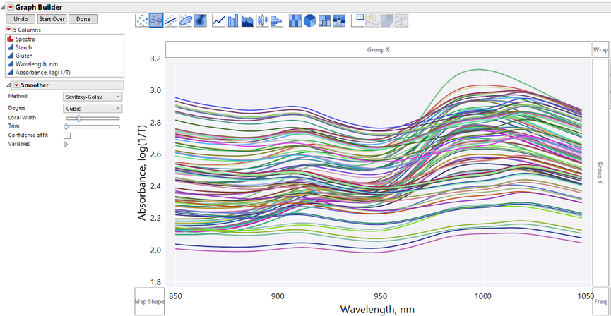
In Graph Builder, there are alternate smoothing methods – such as smoothing splines and LOESS – that you may also want to try out. There are also alternate weight functions in the smoother red triangle menu. Many of these options were newly added in JMP 16.
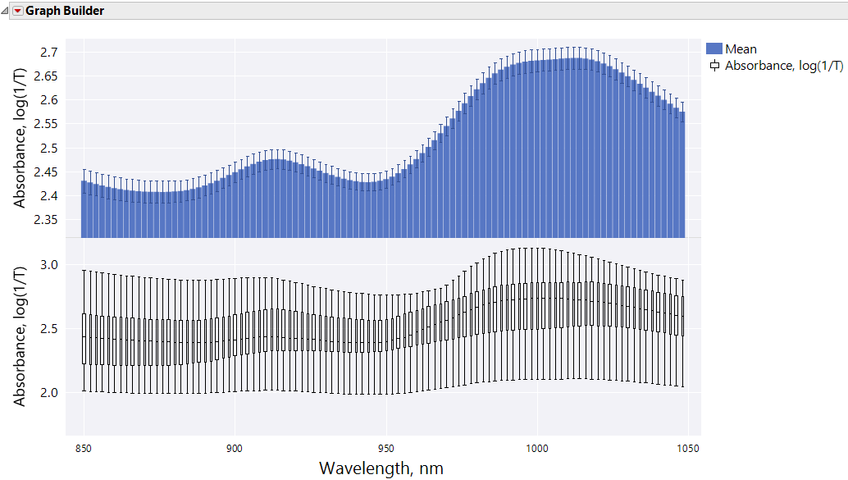
Other summary measures that will quantify the quality of spectra are accessible in Graph Builder. To create these, remove the overlay variable so that the mean spectra is shown. Then, selecting the bar plot and box plot options will generate the plots in Figure 3. Variation that is constant across wavelengths often indicates noise – and a need for further pre-processing – whereas large variation that is specific to certain wavelengths may indicate real chemical effects.
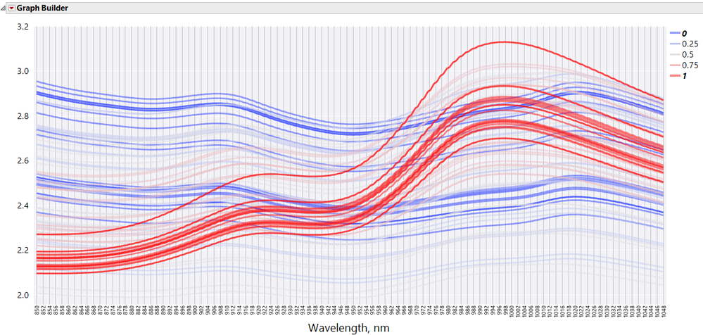
One other type of plot that is useful if your data is in wide format is the parallel plot (Figure 4). This is particularly useful if you are analyzing the spectra in other platforms that require the wide format such as PCA, PLS or other predictive modeling platforms. Selecting spectra in the parallel plot will highlight the corresponding rows in other platforms:
Pre-processing
One of the major stumbling blocks with analyzing spectral data is the need for complex data pre-processing. We will show how using an add-in for Savitsky-Golay derivative filtering and a formula for standard normal variate (SNV) scatter correction can “clean up” your data, making it more easily interpretable and ultimately allowing you to build more reliable predictive models.
For the first step, we will remove the apparent baseline shifts in the spectra. For this, we use a SG data filtering add-in developed by Ian Cox (see the add-in attached to this post below). This will only accept data in a wide format. Choose the “Data Filtering” add-in from the list of installed add-ins in JMP. Select the columns to be manipulated and select OK. Three output graphs will pop up for review.
The SG smoother user interface is where the polynomial order of fit, 2 –
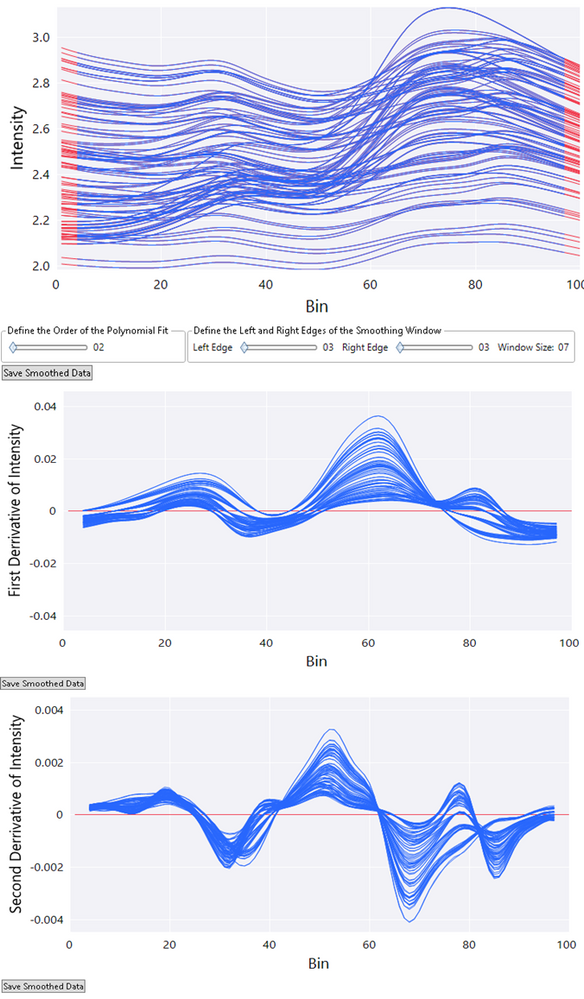
The filtered data can be saved to a new data table, which can then be transferred back to the original data table for further pre-processing if desired. In this case, the first derivative data was selected and saved back to the original data table.
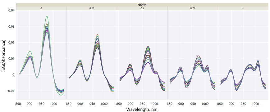
This appeared to effectively remove the baseline shifts. However, there is still some scatter effects remaining in the spectra. One way to visually separate out the scatter effects and chemical effects is to use a grouping variable in Graph Builder. Move the gluten content variable to the one of the group axes. Graph Builder will find a sensible binning and create separate panels for each bin. In these data, we only have 5 values of gluten content. Scatter effects remain because the first derivative removed the additive baseline shift, but did not remove the multiplicative scatter effect. We will show how to illustrate multiplicative scatter effects with a scatter effects plot in the next blog post.
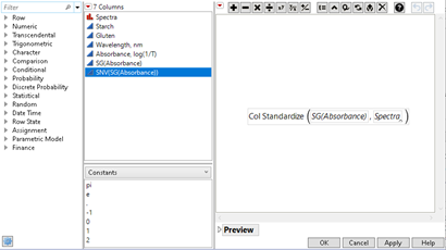
To remove the remaining scatter effect, we perform a SNV standardization. SNV requires the data to be in a stacked format. We create a new column and add the formula shown in Figure 7.
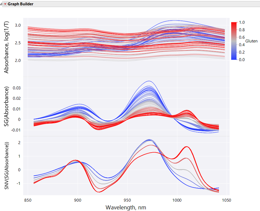
The raw spectra and final pre-processed spectra are shown in Figure 8. To easily launch a plot like this, use the Launch Graph Builder command in Spectra Tools.
These simple steps have already resulted in a much easier to interpret spectra, with baseline shifts and multiplicative scatter effects removed. In their original paper, Martens et al. demonstrated how the more advanced extended multiplicative signal correction can further improve on this pre-processing workflow. We will cover this in the next post.
Future posts
We plan two more posts in this series. The next will show some more advanced pre-processing methods like multiplicative scatter correction and baseline subtraction.
We will also demonstrate how dynamic time warping in Functional Data Explorer can be used to align chromatograms. The final post will apply some of the predictive modeling methods in JMP, such as PCA, PLS, and Generalized Regression, to spectra after pre-processing.
Try some of these approaches out, and let us know how they work with your data!
You must be a registered user to add a comment. If you've already registered, sign in. Otherwise, register and sign in.
- © 2025 JMP Statistical Discovery LLC. All Rights Reserved.
- Terms of Use
- Privacy Statement
- Contact Us
