Time Series Analysis - Seasonal Variation Modeling

rwdavis513 · Feb 5, 2016 06:51 PM

One thing common to almost all manucturing plants is Statistical Process Control. How well a site a consistently make the same product over and over again can be the difference between a mediocer company and a great one. One key to that process is looking for shifts or trends in the data. Although not commonly used, Time Series Analysis can be a helpful tool along the journey of variation reduction.

The time series analysis platform in JMP can be accessed under Analyze > Modeling > Time Series

Let’s take a look at one data from the sample data. Go to Help > Sample Data. Then click on the Time Series drop down and go to Monthly Sales. Open the Time Series platform and select the Sales($1000) column with Date as the Time Series.

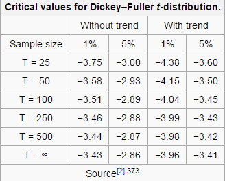
As usual in JMP, right off the bat we have some test statistics to tell us something about this data. Notice the Zero Mean ADF, Single Mean ADF and Trend ADF stats in the table to the right of the graph. ADF stands for Augmented Dickey Fuller test, which is a way to check for a unit root (a feature which changes over time) within the time series. In lamen’s terms, it’s checking for an underlying time dependent trend within the data. The three metrics correspond to checking for no underlying time component (zero mean), constant increase over time (single mean) and acceleration over time (Trend). If the statistic is below the T value found below then the null hypothesis that it is not a component can be rejected. In other words, if it’s below the T value then there is an underlying time component.

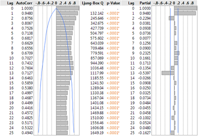
Underneath the first graph you’ll find an AutoCorrelation summary. It shows how each point is dependent on the previous points.

Noticing the clear cyclical pattern could lead one to try a Seasonal Exponential Smoothing Fit to predict the data. Go to the Red Triangle > Smoothing Model > Seasonal Exponential Smoothing.

The red line shows the fit of the model along with the predicted values going into the future. The Model summary has the traditional stats such as DF (Degrees of Fredom), Rsquare, etc. It also includes the Akaike’s ‘A’ Information Criterion (AIC). This metric is great for comparing different models because it penalizes extra parameters in the model so those with extra terms don’t get an unfair advantage. Similarly the Schwarz Bayesian Criterion (BIC) penalizes extra parameters but does so more severly than the AIC. In general, they will agree except when AIC points a higher order model (more complex). For both numbers a lower value is better.

Model Summary

DF		129
Sum of Squared Errors		21565.8785
Variance Estimate		167.177353
Standard Deviation		12.9297082
Akaike's 'A' Information Criterion		1048.48556
Schwarz's Bayesian Criterion		1054.23595
RSquare		0.98719989
RSquare Adj		0.98710066
MAPE		3.44018638
MAE		9.90829917
-2LogLikelihood		1044.48556
Stable	Yes
Invertible	No

Parameter Estimates

Term	Estimate	Std Error	t Ratio	Prob>\|t\|
Level Smoothing Weight	0.2493692 0.0404538 6.16	<.0001*
Seasonal Smoothing Weight	1.0000000 0.0980935 10.19	<.0001*

I hope this helps you in your exploration of time series data. Please leave a comment if you have any questions about time series analysis or any great Time Series stories to share. Thanks!