A cubic spline is a smooth, continuous function that represents the relationship between two numeric variables. It consists of a series of third-order polynomials fit together in a piecewise fashion, under the condition that the function is continuous and differentiable at the knots, or connection points.
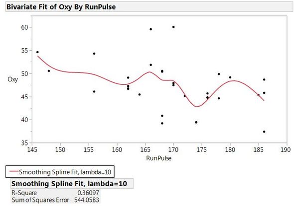
JMP offers spline fits in the Fit Y by X platform. For example, using the Fitness.jmp sample data table, I can fit a cubic spline for the Oxy column by the RunPulse column.
 Spline Fit of Oxy by RunPulse
You can get the coefficients of the polynomial functions by clicking the inverted red arrow hot-spot for “Smoothing Spline Fit” and selecting “Save Coefficients”. A new data table is generated containing an X column that gives the “RunPulse” values (in this case) that are taken as the knots where the individual cubic polynomial functions are connected. The remaining columns in the data table are the coefficients for each cubic spline: “A” is the intercept term, “B” is the coefficient for the linear term, “C” is the coefficient for the quadratic term, and “D” is the term for the cubic term for the variable (X-O) where O is the value of the knot at the beginning of the interval:

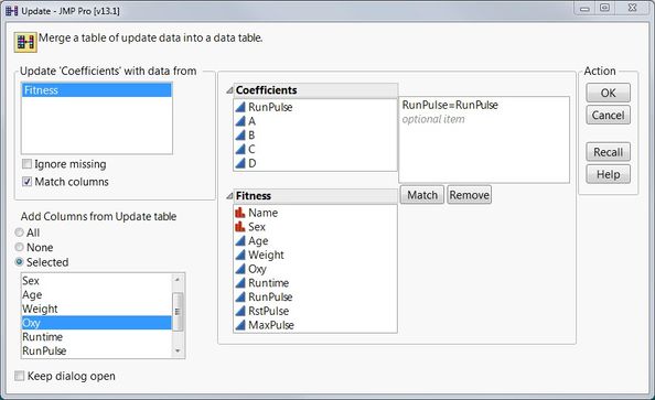
To better understand the concept of the spline fit, I updated the coefficients table to include “Oxy” values using the "Tables->Update" option:
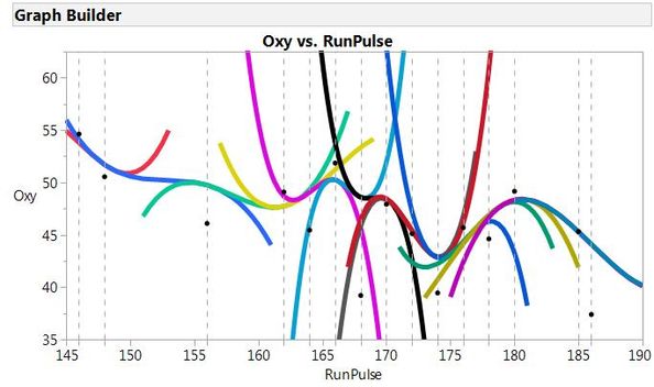
 Updating the Coefficients tableThen I recreated the spline fit using the coefficients, extending the polynomials beyond the knot points:
 All cubic polynomial functions used to fit the spline
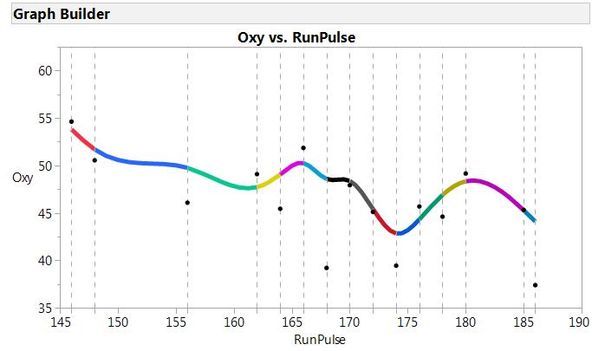
The points and dashed vertical lines show the knot points, and the individual polynomial curves are represented by different colors. Finally, you can see the spline fit itself when the polynomials are truncated at the knots:
 Truncated cubic polynomial functions defining the splineHere, you can see each segment of the final cubic spline, and how they are connected together. Hopefully, this explanation will take any mystery out of cubic splines and help to understand this smoothing fit.