In the first blog post in my nonlinear modeling series, I explained what nonlinear modeling is. Here, I show you how easy it is in JMP.
Fit Curve in JMP 13 enables you to specify the X and Y variables for a model and choose the general form of the model. JMP then fits the chosen model automatically. You do not need to specify the starting values of the parameters. Fit Curve includes sigmoid curves, exponential growth and decay models, peak models, pharmacokinetic models, and the Michaelis Menten model. The platform also includes the ability to fit separate models for the levels of a grouping variable and then compare parameter estimates and test for parallelism. JMP gives you fit statistics that allow you to compare different models that are fit to the data.
To illustrate the Fit Curve platform, we will examine data collected when studying the drug theophylline using a one compartment oral dose model (see data attached to this post). Theophylline is used as a long term medication to control lung disease. In order to regulate the dose of the medication, researchers measured the concentration of theophylline in the bloodstream. They want to determine the relationship between the concentration and the time after ingesting the drug. The drug was administered to 12 patients, measuring the theophylline level eleven times for each patient. The subject identifier, time, and concentration of theophylline were recorded.
To use the Fit Curve platform to fit the model to the data, select Analyze --> Specialized Modeling --> Fit Curve. (Note: Prior to JMP 13, the Fit Curve platform was part of the Nonlinear platform and was accessed by selecting Analyze --> Modeling --> Nonlinear and assigning a column without a formula to the X role). Assign concentration to the Y role and time to the X role. In this case, use subject in the Group role to fit separate models for each of the subjects in the study. This will allow you to compare the model parameters between subjects. Select OK and graphs of the data are displayed.
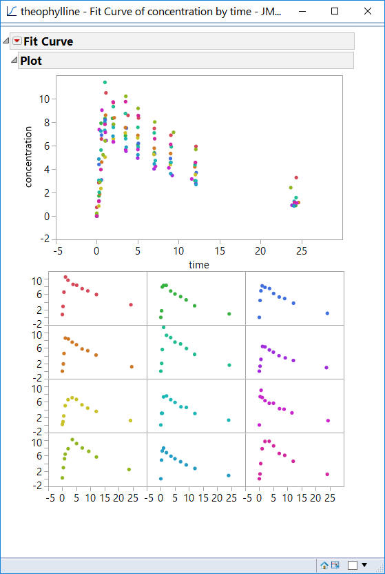
To fit the model of interest, click on the red triangle at the top of the report window. Select Pharmacokinetic Models --> Fit One Compartment Oral Dose. The results include the Prediction Model, Summary of Fit, Parameter Estimates, and Plot.
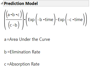
The Prediction Model displays the model formula, including the parameters. When appropriate, physical interpretation of the parameters is also shown. In the case of the one compartment oral dose model, the parameters represent the area under the curve, the elimination rate, and the absorption rate.
The summary of fit statistics are provided both within the model results and in the Model Comparison section at the top of the report. In cases where multiple models are fit to the same data table, the summary of fit statistics for all models fit in the window will be shown in the Model Comparison report.
For this model, there are three parameters estimated for each of the subjects. Analysis of means can be used to compare the parameters across subjects. To generate the analysis of means decision charts, click on the red triangle next to the model name and select Compare Parameter Estimates.
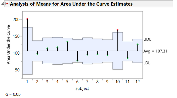
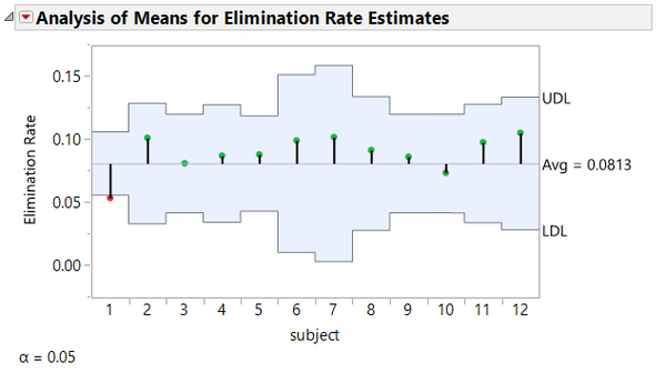
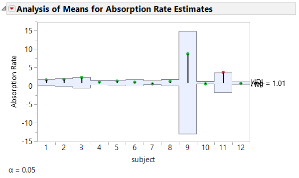
On the analysis of means plots, any point that is outside the shaded area is considered statistically different from the others at the 0.05 level of significance. These statistically different points are also red rather than green. For each category of parameter estimates there is at least one subject for whom the parameter estimate is found to be statistically different than the others. For example, in the last plot shown, the absorption rate estimate for subject 11 is different than the estimates for the other subjects. This is an indication that a single model may not be appropriate for this data. It may also prompt additional examination of patients 1, 10, and 11 to see if there is a particular demographic or medical history reason that they are different from the other subjects.
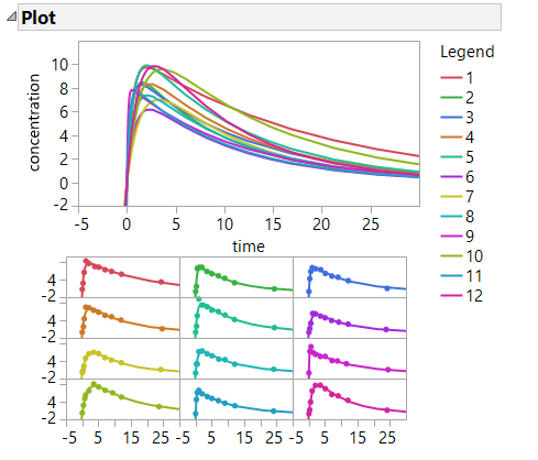
A series of plots are also provided to illustrate the models that are fit. There is a single plot that overlays all of the subjects, and a matrix of plots that shows each patient individually.
A second example
Another type of model that can be fit with Fit Curve is a growth model. Consider the relationship between concentration and velocity for a particular enzyme/substrate pair. The reaction rates (velocity) are observed at different substrate concentrations.
To begin, select Analyze --> Specialized Modeling --> Fit Curve. Assign Velocity as the Y variable and Concentration as the X variable. After selecting OK, examine the plot of the data.
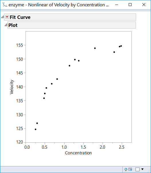
At first glance, one might consider fitting a quadratic model to this data. While a quadratic model is not nonlinear, such polynomial models are included in Fit Curve for ease of comparison. Fit a quadratic model by selecting Polynomials --> Fit Quadratic from the red triangle menu.
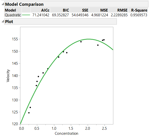
The R-Square statistic is quite high. However, you might be concerned about the predicted velocity beginning to decline at a certain point in time. Assuming that this decline is not possible in this circumstance, a growth model might be more appropriate. Fit both mechanistic growth and Michaelis Menten models to the data by selecting Exponential Growth and Decay --> Fit Mechanistic Growth (and Fit Michaelis Menten) from the red triangle menu. Examine the results.
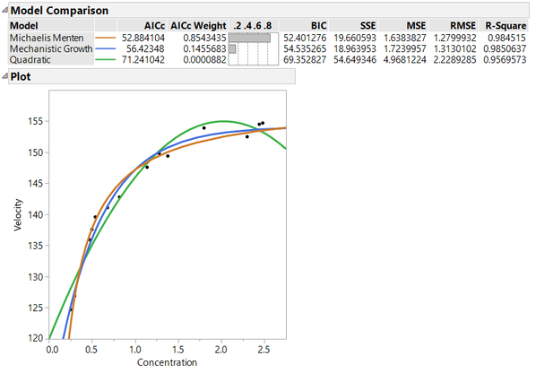
The plot now has all three models superimposed. Analysts often use either the AICc (Akaike Information Criteria corrected [for sample size]) or BIC (Bayesian Information Criteria) statistic to compare the models. For both of these criteria, smaller values indicate a better model. Each of these statistics is a measure of model fit with a penalty imposed for more parameters in the model. Using either of these statistics, the Michaelis Menten model would be considered to be the best model. The AICc weight can also be used for comparison purposes as a measure of how much better one model is compared to the others. The AICc weight is defined as:
AICcWeight = {exp[-0.5(AICc - AICcBest)]}/AICcSum
Where AICcBest is the smallest AICc among the fitted models, AICc is the AICc statistic for the current model, and AICcSum is the sum of the AICc’s for all of the fitted models. The AICc weight is the probability that the model is the “right” model given that one of the fitted models is in fact the right model. In this example, there is an 85% chance that the Michaelis Menten model is correct under the assumption that one of the three models fit is the correct model.
The Fit Curve platform is excellent at generating the model equation, providing starting values for the parameters, and generally solving for the parameters. But…what happens if you want to fit a model that is not included in the Fit Curve arsenal? Part 3 will focus on the Model Library in the Nonlinear platform.
Editor's note: Check out the whole four-part series.