- JMP User Community
- :
- Blogs
- :
- JMPer Cable
- :
- Is it uniform?
- Subscribe to RSS Feed
- Mark as New
- Mark as Read
- Bookmark
- Subscribe
- Printer Friendly Page
- Report Inappropriate Content
José G. Ramírez @ZenEos, Ph.D., W.L. Gore and Associates, Inc.
NOTE: This article originally appeared in JMPer Cable, Issue 27, Winter 2011. The author recently co-authored with Brenda Ramirez a SAS Press Book, Douglas Montgomery's Introduction to Statistical Quality Control: A JMP® Companion.
If you have taken a basic course in probability and statistics you were probably introduced to the Uniform distribution. Don’t blame yourself if it isn’t foremost in your memory; the Uniform distribution doesn’t have much appeal because it describes a phenomenon with constant probability. It seems hard to find applications in engineering and science for which the probability of occurrence is constant for all the values in a given interval. Pseudo-random numbers between 0 and 1 come to mind since any number in this interval should have the same probability of occurring. The Uniform distribution has sometimes been used as a model for the distribution of traffic along a straight road.
In general, probability distributions are mathematical models, or equations, used to describe and quantify the degree of uncertainty that we observe in our data. Under a continuous uniform probability model, the likelihood of observing a value x in the interval [θ,θ + σ] is constant and equal to, 1/σ or 1 divided by length of the interval. The mathematical equation describing a continuous uniform (rectangular) probability density function is

One of the readers of our blog, StatInsights, asked how to fit a Uniform distribution in JMP. Uniform is not one of the choices in the Continuous Fit contextual menu of the Distribution platform. However, Beta is one of the choices.
Uniform (θ,θ + σ) is Beta (1, 1,θ, σ).
Fortunately, there is a convenient relationship between a Beta distribution, which is one of the JMP choices, and the Uniform distribution. The general form of the Beta probability density function is
where B(α,β) is the Beta function. This pdf generalizes the standard 2-parameter Beta distribution, Beta(α,β), from the interval [0,1] to an arbitrary bounded interval [θ,θ + σ]. When the shape parameter values are α= 1 and β = 1, then the beta function B(1, 1) = 1 and the pdf has constant probability equal to 1/σ. In other words, if X is distributed as uniform in the interval (θ,θ + σ), then X is distributed as Beta(1, 1) with threshold θ and scale σ.
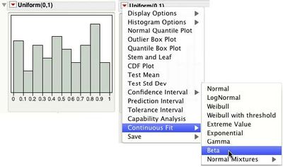
Let’s explore this relationship. The histogram in Figure 1 shows 100 simulated observations from a Uniform distribution in the interval (0,1). These observations were generated using the Random Uniform generator in the Formula Editor.
As expected, this distribution has a somewhat rectangular shape. To fit a Uniform distribution to this data, select Continuous Fit > Beta from the contextual menu (red triangle) on the histogram Uniform(0, 1) title bar.

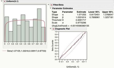
Figure 2 shows the histogram with the superimposed Beta fit, which has a rectangular shape. The fitted Beta Parameters Estimates show α=1.07 and β=1.03 (close to 1 — but how close?). The 95% confidence intervals for α and β both include 1, indicating that there is not enough evidence to say that they are different from 1. In practical terms, that means α and β are assumed to be 1 so the Uniform distribution does a good job at describing this data. The threshold parameter, θ, is 0.009 and scale parameter, σ, is 0.977 supporting a Uniform(0, 1). (Note that θ and σ are not maximum likelihood estimates. JMP sets θ to the minimum data value, and σ to the range (=maximum-minimum) of the data). Finally the Diagnostic Plot shows the points hovering closely around the line, and within the 95% confidence bands.

For a Uniform(θ, θ + σ), the mean is equal to θ + σ/2 and the standard deviation is equal to σ/√12 . The Moments table in Figure 3 shows the mean to be close to 0.5 and the standard deviation to be close to 1/√12 = 0.2886. Both the 95% confidence intervals for the mean and standard deviation contain 0.5 and 0.2886, respectively.

What to Look for When Fitting the Beta(1, 1, θ, σ)) To use the beta distribution fit to see if the Uniform distribution is a good approximation for data, follow these steps.
- Fit a Beta distribution in the Distribution Select Continuous Fit > Beta from the red triangle menu on the Histogram title bar.
- Look at the Parameter Estimates report and verify that the estimates for the shape parameters α and β are close to
- Verify that the 95% confidence intervals for α and β include 1.
- Select Diagnostic Plot from the red triangle menu on the Fitted Beta title bar. The points on the diagnostic plot should fall close to the straigh
- The Uniform(θ, θ + σ) parameters are given by the threshold θ and scale σ.
- Select Confidence Intervals > .95 from the red triangle menu on the Histogram to see 95% confidence intervals for the mean and standard deviation (see Figure 3).
- Check that θ + σ/2 (mean) and σ/√12 ( Dev.) are within the intervals.
Example: The Brisbane Baby Boom Data > December 18, 1997, was a record-breaking day for Brisbane in Queensland, Australia. Forty-four babies were born in a 24-hour period at the Mater Mothers' Hospital.
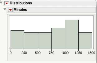
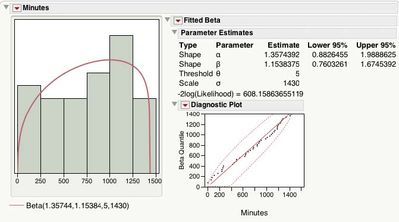
Figure 4 shows the histogram of the number of minutes since midnight for each birth occurring that day. It is reasonable to believe that in a 24-hour period a birth can occur at any minute, and the histogram seems to support that. Will a Uniform distribution fit the data well?


Figure 6 shows the moments and 95% confidence intervals for the mean and standard deviation. For a Uniform(5, 1435) the mean should be close to 5 + 1430/2 = 720, and standard deviation close to 1450/√12 = 412.8054. The 95% confidence interval for the mean does contain 720, and the one for the standard deviation contains 412.8054.

Next time you are wondering if your data can be described by a Uniform distribution, think ‘beta’ and use the Distribution platform with Continuous Fit > Beta fit.
- © 2024 JMP Statistical Discovery LLC. All Rights Reserved.
- Terms of Use
- Privacy Statement
- About JMP
- JMP Software
- JMP User Community
- Contact


You must be a registered user to add a comment. If you've already registered, sign in. Otherwise, register and sign in.