- New to JMP? Let the Data Analysis Director guide you through selecting an analysis task, an analysis goal, and a data type. Available now in the JMP Marketplace!
- See how to install JMP Marketplace extensions to customize and enhance JMP.
JMPer Cable
A technical blog for JMP users of all levels, full of how-to's, tips and tricks, and detailed information on JMP features- JMP User Community
- :
- Blogs
- :
- JMPer Cable
- :
- Geocoding 2020 add-in
- Subscribe to RSS Feed
- Mark as New
- Mark as Read
- Bookmark
- Subscribe
- Printer Friendly Page
- Report Inappropriate Content
Geocoding has been around for some time. But now, this service is offered via REST interfaces which provide more flexibility and accuracy. I created an add-in that uses the service from Mapquest to find geo-codes for addresses and calculate distances, traveling times or complete routes between pairs of locations. This is the description of its functionality and usage.
I’ve always been fascinated by maps. Before digital maps became available, I bought maps for every vacation, usually in different scales and in much greater detail than I really needed. So, it should come as no surprise that I am also fascinated by JMP’s graph features that allow data to be represented on maps.
What is geocoding?
One of the interesting applications is geocoding, or the ability to locate points on maps. Usually, you have a point of interest and its address. To find its position and plot it on a map, you also need the geocoordinates. As you might expect, Wikipedia offers more details on geocoding.
Why a new geocoding add-in?
In recent years, computer communication technique known as REST has become more widely used. In a 2019 keynote, John Sall talked about the “Secret Features of JMP.” One of these hidden gems in JMP is really buried quite deep: the ability to access the REST APIs (advance programming interfaces) through JSL commands. Since computer communication data are often exchanged using the “JSON” data structure, JMP developers created JSL commands that transfer data between JSL data structures and JSON data with ease. This technique has become increasingly important. In fact, Johns Hopkins University and the Robert Koch Institut offer REST APIs for their data pools for information related to COVID-19; JMP customers use them to access SAP data for quality management; and I use one for geocoding. This interface extends the possibilities of information exchange, since it provides more than the geocoordinates of points of interest. It also allows users to get information about distances, traveling times and even routing. This article is about the usage of the add-in that I loaded into the file exchange. Technical background will be given in separate post, as summarized in the last paragraph.
What are the functions?
You need a data table with address information per observation. The addresses can be used to add three different levels of geo information, where every level contains the information of the previous one.
- Geocoordinates
For every observation, the latitude and longitude of its location is added. In addition, you will get the hierarchy of administrative units, country, state, district, postal code, city, street and an assessment of how close that address has been hit, as far as the information available in the database.
- Distance and traveling time
For every pair of consecutive rows in your data table (e.g., row 1 –> row 2 / row 2 –> row 3 /….), the distance between the addresses and the required travelling time will be added to the second row. The connections become enumerated in an extra column. The traveling time is calculated based upon the user’s choice of transportation: car, bike or walking.
- Routing
An additional table is created that contains all the above information, as well as the geocodes of all points that describe the route between two consecutive rows.
Presuppositions
There are several internet sites that offer mapping and routing services. A good overview is given by the journal ProgrammableWeb. I decided to use MapQuest. The company offers a variety of paid services but also a free API. If you want to use it, you need to register first and get a free API key. Of course, you also need the Geocoding 2020 add-in. It will install itself in the Add-Ins menu in the “Map Shapes” submenu.
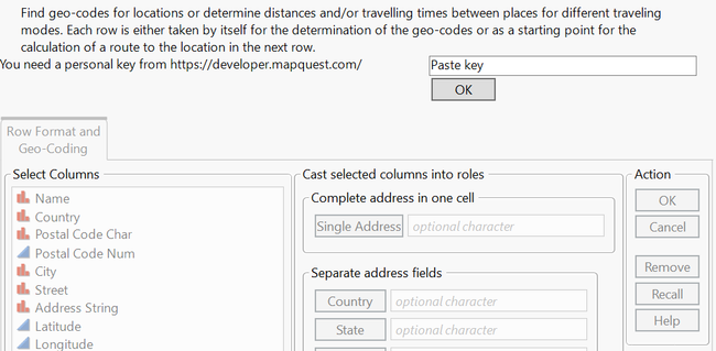
Upon the first call, you will be informed that you can get the necessary key from MapQuest and provided a field to paste in the key.
The reminder of the dialog is disabled. After the key is pasted, it is tested to determine if it is a proper MapQuest key; the key must be verified before you can proceed. If you provided a valid key, it is saved in the user’s directory in folder AppData/Roaming/SAS/JMP. If this directory does not exist, it will be created.
For all of the commands in the add-in to work, you must set the JMP language to English and select the “Use JMP language…” option. Unfortunately, that can’t be done via JSL. You must make these selections using your language equivalence to File -> Preferences -> Windows specific. The add-in will verify that the language settings are correct and will alert you if that is not the case.
Let’s go
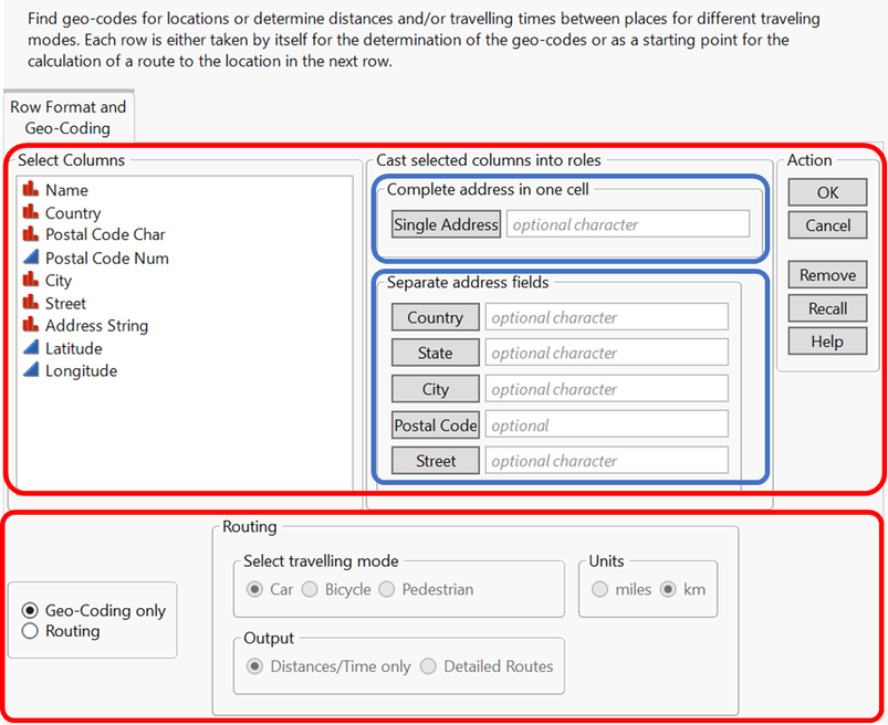
The menu consists of two parts. The first part is the upper red area, which is built like nearly all JMP platform dialogs; it contains the column list, the role part and the action panel. In the role area, there are two parts, emphasized by blue frames. In your data table, the address information may be stored in one of two formats: either as one column that holds the complete address as a text string, or as separate columns, with each column holding a part of the address like country, city, street. You can provide either of these formats, but they are mutually exclusive. In both cases, your address must contain the country. It can be given as name or as an ISO code, whichever you prefer.
The second part is the lower red frame that shows which options are available. They are organized in groups of radio buttons (the screen shot below shows the defaults). All options add a group of additional columns to your data table; the combination of “Routing” and “Detailed Routes” creates an additional data set with a copy of your data. These points are identified as “Points of Interest.” In addition, there are “Waypoints,” the points that need turns along your route.
An example
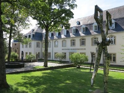
To test how it all works, I gathered some address information from the internet. I grew up in Solingen, a small town in the western part of Germany. It was well-known during medieval times for producing high-quality swords and cutlery, which is why you’ll find the German Museum of Cutlery here. Next to the museum is a small but very impressive baroque church. There are also some other famous places nearby:
|
Deutsches Klingenmuseum |
German Museum of Cutlery |

|
Gräfrather Klosterkirche |
Baroque monastery church |

|
Das Neandertal |
The region where the remains of a branch of our ancestors were first discovered |
|
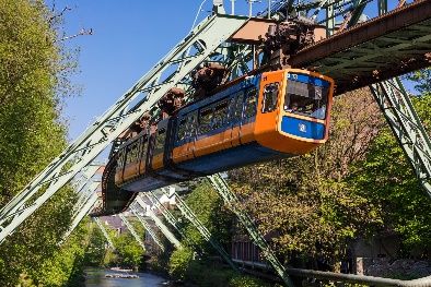
Die Wuppertaler Schwebebahn |
A 13-km-long suspension railway, the oldest electric elevated railway with hanging cars in the world, inaugurated in 1901 |
|
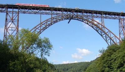
Die Müngstner Brücke |
The highest railway bridge in Germany, built in 1897 |
|
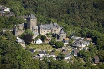
Schloss Burg |
A reconstructed castle, originating from the 12th century |
After searching the internet for the addresses, I copied the strings into a JMP data table. None of the addresses included a country name, so I prepended “Deutschland, ” to all the strings. The strings now look like this
|
Deutschland, Talstraße 300, 40822 Mettmann |
|
Deutschland, Alte Freiheit 24a, 42103 Wuppertal |
|
Deutschland, Klosterhof 4, 42653 Solingen |
|
Deutschland, Klosterhof 3, 42653 Solingen |
|
Deutschland, Müngstener Brückenweg, 42659 Solingen |
|
Deutschland, Schloßplatz 2, 42659 Solingen |
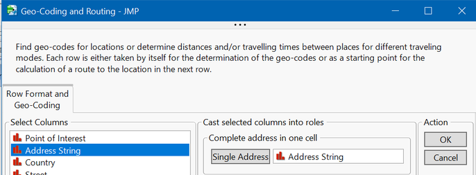
I choose the German country name “Deutschland” on purpose. In the dialog, assign this column to the “Single Address” role and go.
As result of the run, these columns are appended to your data set:
|
Geo-Information |
|
GC#Latitude |
|
GC#Longitude |
|
GC#Country Code |
|
GC#State |
|
GC#District |
|
GC#Postal Code |
|
GC#City |
|
GC#Street |
|
GC#Quality Assessment |
|
GC#Return Message |
I think that the column names speak for themselves. MapQuest provides an estimated quality rating for each hit. It is quite elaborate, so I summarized that information into four categories: Exact, Close, Approximate, Far. The rows in your data table get symbols and colors according to this rating. All positions are displayed in a map, and a script that reproduces this map is added to the data table. Depending upon the area over which your points are distributed, the background map is either Street Map or Simple Earth.
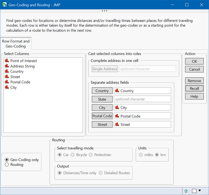
In that data table, I split the address string into its single components (it’s easy if you use Cols à Utilities à Text to Column…) and requested the coordinates using the “Separate address fields” roles.
There is no need to fill all the role fields in this section. Country is a minimum requirement. The more information you provide, the better the hit rate. Results from both methods for requesting coordinates are not completely identical. The coordinates themselves may deviate a little bit and for the detailed request, more information (such as district) may be given. The quality assessment may vary as well.
For performance reasons, single address fields are concatenated to one string and single string requests are sent to MapQuest if there are more than 200 addresses in your data table.
If you choose the combination of “Routing” and “Distances/Time only,” you will get the same information back as for geocoding, plus three additional columns. From time to time, you may receive error messages:
|
Point of Interest |
GC#Return Message |
GC#Distance (km) |
GC#Time (Bicycle) |
GC#Legs |
|
Neandertal |
|
. |
. |
0 |
|
Wuppertaler Schwebebahn |
Unable to calculate route. |
19.1287 |
:0:00:52:39 |
1 |
|
Deutsches Klingenmuseum |
Unable to calculate route. |
0 |
:0:00:00:00 |
2 |
|
Gräfrather Klosterkirche |
|
0 |
:0:00:00:00 |
3 |
|
Müngstner Brücke |
|
9.92 |
:0:00:26:26 |
4 |
|
Schloss Burg |
|
5.0163 |
:0:00:13:55 |
5 |
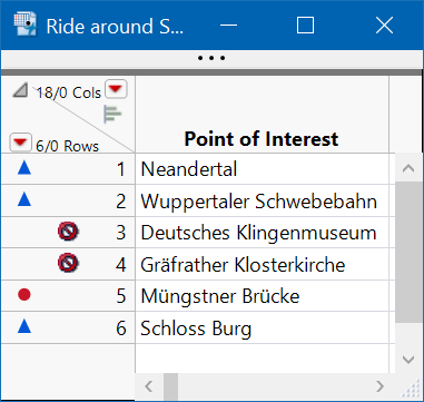
Consecutive rows build one leg of the total route. The target row holds the information of the leg. In the example, the first leg is from Neandertal to Wuppertaler Schwebebahn. The distance for a bicycle route is roughly 19 kilometers, and the estimated cycling time is 52 minutes.
For whatever reasons, cycling routes could not be found to Deutsches Klingenmuseum or Gräfrather Klosterkirche. Therefore, legs two and three have no travel information, while legs four and five provide the respective information again.
This combination of options requests details for a route between two consecutive rows in the data table with distances given in miles:

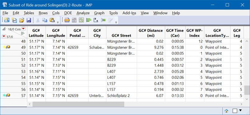
Row 49 holds the next-to-last address in the data table, which is where leg 4 ends. The route leading from the place before to this point was 9.3 miles long and has an estimated travelling time of 15 minutes by car. It is a “Point of Interest.” The next row is the end of the first segment of leg 5 after +/- 300 feet and five seconds of driving time. It is the first waypoint in a series of seven, before the next (and last) point of interest is reached. Maps show the results, and their scripts are in the tables as well.
The data table is part of the add-in and can be opened using the “Help” button. You may use it to start playing around and looking at the pictures of the attractions that I included.
And if you should ever come to this area and visit some of the places, don’t forget to look for a restaurant that serves Bergische Kaffeetafel, a very rich combination of local specialties including bread, sausages, sweet rice, waffles and more. It’s well-known all around the area that I picked as a demonstration, so you should be able to find it at many restaurants.
At the first run
MapQuest requires you to have a personal API key. You get it from their developer’s website for free. The add-in asks for this key and provides a field to paste it into.
The add-in stores the key in the user’s appdata directory for SAS\JMP. Before every run, it tries to read the key and will use it as long as it’s there.
Excluded rows/routing not possible
The add-in assigns symbols, colors and labels to the rows, but it also respects the “excluded” row state, which has specific consequences for the routing application. If a row is excluded or routing to its address is not possible, then this row is ignored and a route to the next address is searched for.
In this situation, routes between Neandertal and Wuppertaler Schwebebahn, between Wuppertaler Schwebebahn and Müngstner Brücke and between Müngstner Brücke and Schloss Burg will be searched.
Similarly, locations will be skipped if routing to them is not possible.
Technical details
The attentive observer may have noticed that the main dialog is contained in a tab. Tabs are useless if they stand alone. This tab reflects the idea that locations for routings may appear in different formats. If there should be requests for alternative ways of providing locations for routing, that tab may get siblings.
I was motivated to write this add-in as a result of my combined interest in maps in general and the REST API technique. To make the latter one more transparent and perhaps even more widely used, I put three files into the JSL cookbook. They are defining functions that can be called by other programs. One is the REST call to MapQuest. I describe content and a description of the interface in a blog post about the crude MapQuest call. The other scripts are envelopes for the REST call. They take JMP lists as inputs and build the JSON structures that are needed for the geocoding or routing call. If there are many addresses to be coded, it packages them into blocks of 50 for better reliability and performance. In my blog posts about the geocoding and the routing subroutines, I describe these pieces of code in greater detail.
As mentioned before, JMP programmers did a great job of providing JSL functions that translate in both directions between JMP data structures and JSON. In JSL terms, there are lists and associative arrays involved. These elements can be stacked. You may have an associative array that contains a list of associative arrays that contains… . A single MapQuest call delivers a rich set of data from which I only needed some of the elements. Sometimes, these were two levels deep in the stack; other times, many levels deep. So, I found it useful to write a little script that iterates through this structure. And I would not be a respectable JMPer if I didn’t look for a visualization of the result. I found the perfect way in the Ishikawa diagram. Programming this reminded me of the power of recursion, which is the best technique to step down a deep stack and return safely. I thought it might help or inspire other programmers as well. I put the script into the cookbook and – naturally – I wrote a post about recurse and draw hierarchical structures.
I used JMP 15 for the development, using a JMP Project. I wouldn’t say that my little project couldn’t have taken place without Projects, but Projects made it a lot easier.
You must be a registered user to add a comment. If you've already registered, sign in. Otherwise, register and sign in.
- © 2026 JMP Statistical Discovery LLC. All Rights Reserved.
- Terms of Use
- Privacy Statement
- Contact Us

