- JMP User Community
- :
- Blogs
- :
- JMP Blog
- :
- Why design experiments? Reason 5: Complex behaviours
- Subscribe to RSS Feed
- Mark as New
- Mark as Read
- Bookmark
- Subscribe
- Printer Friendly Page
- Report Inappropriate Content
I want to demystify design of experiments (DoE) with simple explanations of some of the terms and concepts that can be confusing for people when they are starting out. As an illustration, we have been looking at a real-life case study in which we need to understand how to set the Large Volume Injector (LVI) in a GC-MS analysis system. The objective is to optimise detection of low levels of contaminants in water samples.
In the previous post in the series, we saw how the 26-run experiment that we introduced is almost uniquely able to provide clarity about important behaviours of this system.
In this post, we will see how the same experiment can also be used to understand more complex behaviours: interactions.
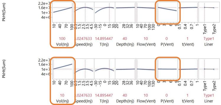
The concept of interactions was introduced in the second post in the series where we saw the understanding you can get from visual and statistical models of your process using experimental data. The Profiler plot of a statistical model of the data, below, shows an interaction of two of the factors: the effect of Vent Pressure depends on the setting of Injection Volume.
If an Injection Volume of 100 µL is used, increasing Vent Pressure has a negative effect on PkHt(Sum). If Injection Volume is set at 10 µL, Vent Pressure has almost no effect on the response.
Can't we just ignore interactions?
If we don’t understand interactions, we don’t understand our process, and we will struggle to find the best settings. In this example, the largest peaks are with high Injection Volume and low Vent Pressure. We wouldn’t know that if we didn’t understand the interaction of these factors.
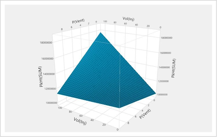
We can also see this interaction by looking at the surface plot, below, of the model with PkHt(SUM) on the vertical axis and the two factors on the horizontal axes.
This illustrates the importance of thoroughly exploring the possibility space. We can only understand this behaviour by testing combinations that cover the extremes of the possibilities. If we had only experimented with P(Vent) set at the highest setting in the range, we would have concluded that Vol(Inj) has little effect on PkHt(SUM). This is one of the disadvantages of one-factor-at-a-time or OFAT experimentation.
Understanding interactions is also important in understanding robustness. From the surface plot, you can see that the settings with the highest PkHt(SUM) are at the top of a steep slope on the surface. If we decide to run the method at these settings but have poor control, such that the actual settings vary about the desired values, we will see large variations in the response. In the opposite corner of the possibility space, PkHt(SUM) is lower, but we are on the flattest region of surface. If being robust to changes in the factors is more important than maximising the response, we would favour these settings of the system.
Experiments and Models to Understand Interactions
Understanding interactions is important. How do we model these interactions?
One way to think about interactions is that they are synergistic effects. They are behaviours beyond the addition of the individual effects of the factors. We can therefore model these as the product of factors. For example, the interaction effect of Injection Volume and Vent Pressure is modelled by fitting the response, PkHt(SUM), to Vol(Inj)*P(Vent). These effects can describe synergistic and anti-synergistic behaviours. In our example, Vol(Inj)*P(Vent) has a negative parameter in the model because the effect is anti-synergistic: We saw in the Profiler plot that as the setting of one factor increases, the effect of increasing the other factor becomes more negative.
How does our 26-run experiment help us to understand interactions? In the previous post, we saw that if we want to understand our process with the most clarity we want the minimum correlation of effects in the experiment. We found that our experiment was good because it has little correlation between main and quadratic effects. What about the interaction effects?
We will only consider the interactions between two factors: two-way or two-factor interactions. In practise, important interactions involving three or more factors are rare. In our example with eight factors, there are still quite a lot of possible two-factor interactions. Let’s count them.
- There are seven interactions with the first factor as it can interact with each of the other seven factors.
- The second factor can interact with six other factors, in addition to the interaction with the first factor that we have already counted.
- The third factor can interact with five other factors, in addition to the first two factors.
- And so on…
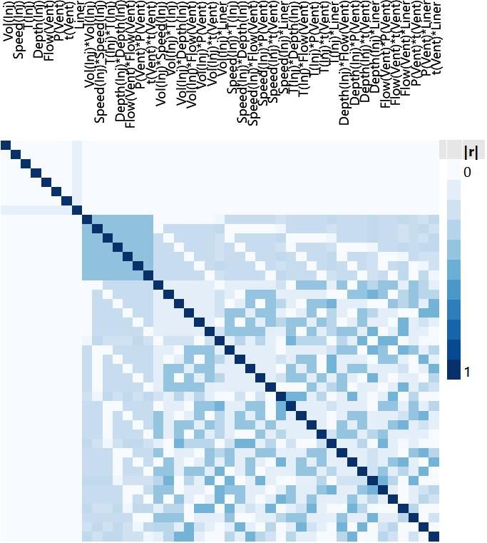
The number of two-factor interactions for our eight-factor example is therefore 7 + 6 + 5 + 4 + 3 + 2 + 1 = 28. To see how well we can understand all of these interactions, we can look at the correlation colour map.
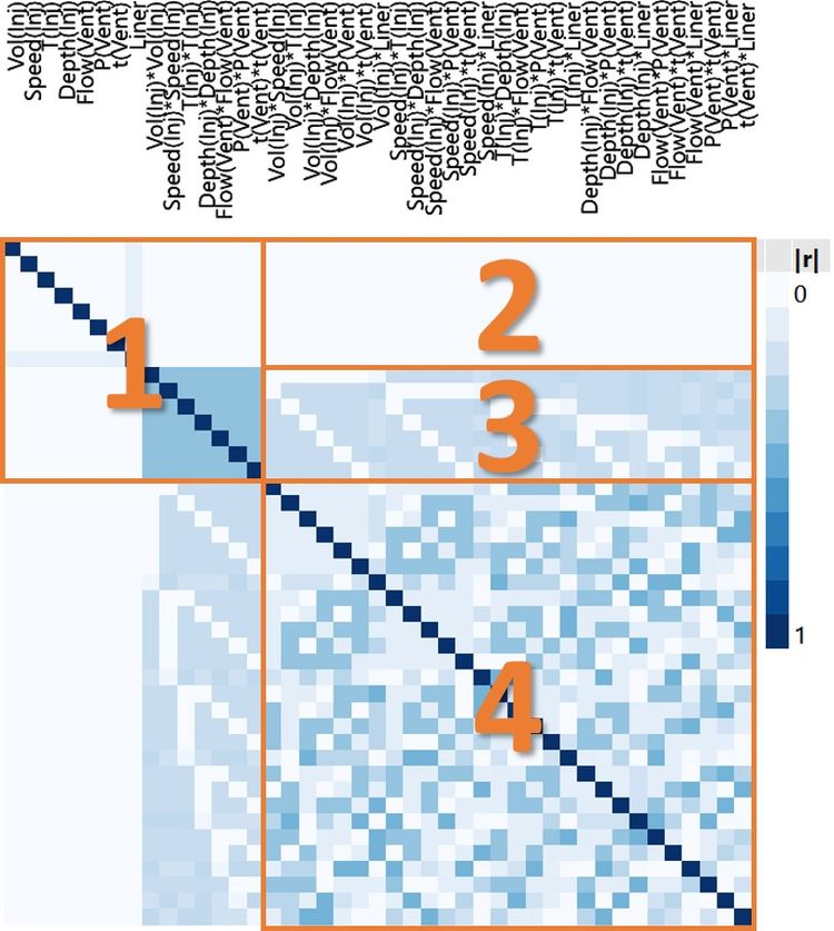
Now that we are also considering the two-factor interactions, we have a lot more to take in. If we break it down, there are some simple insights that we can take from this. I’ve added some labels in the version below to help explain what we are seeing.
Looking at the four labelled regions of this colour map tells us:
- The correlation between main and quadratic effects. We have already seen this in the previous post in this series.
- There is 0 correlation between the eight main effects and our 28 two-factor interaction effects.
- There is minimal correlation between the seven quadratic effects and the 28 two-factor interaction effects.
- Correlations between each of the 28 two-factor interactions and the other 27 two-factor interactions are in the range 0 to 0.48.
From this colour map, we see that we can understand the main effects of our factors with clarity because they are not correlated with the quadratic or two-factor interactions (together we would call these the second-order effects). We will also be able to estimate any important second-order effects because there is no confounding between any of them. And all in relatively few runs.
Back in the first post in this series, we asked why we should choose these 26 runs out of the 4374 possibilities in the full factorial. Now we can see why. You would have to be really lucky to find such useful properties just by choosing runs at random. We ensured that the data would have these properties by creating the plan of runs according to a definitive screening design or DSD approach. Using DoE software like JMP, we can create a DSD for any number of continuous and two-level categorical factors. More generally, we can use DoE software to design a collection of runs with properties to fit our scientific or engineering challenge.
Supersaturation -- Do we need to find a bigger meeting room?
We call the model with all main, quadratic and two-factor interactions effects the full response surface model. It has been found that the response surface model is a useful approximation to behaviours in physical, chemical and biological systems. However, there is a problem here. Remember back to the third post in this series. We said that you need at least one run per parameter in your model. The full response surface model for our example has:
- one intercept.
- eight main effects.
- seven quadratic effects.
- 28 two-factor interaction effects.
This is a total of 44 parameters to be estimated from just 26 runs. We say that the experiment is supersaturated for the response surface model. (It would be just saturated if we had the same number of parameters to estimate as we have runs.)
The minimum number of runs for a DSD for this situation is actually 18. We decided to use the option of eight additional runs to increase the power of our experiment. However, we still do not have enough runs to fit the full model. It is like inviting 20 people to a meeting in a room with only 12 seats.
There is a solution to this seemingly intractable problem and it is not to make eight people stand up. To continue the meeting analogy, suppose you have good reason to think that most of the people you invite will not turn up. There is a parallel here: Most of the time, we find that a lot of the effects are so small that they are not important. We call this effect sparsity.
In the next and penultimate post in the series, you will see how we can bring simplicity to our understanding of processes and systems by finding useful models with only the most important effects.
Have you missed any posts in this series on Why DoE? No problem. See the whole series here.
- © 2024 JMP Statistical Discovery LLC. All Rights Reserved.
- Terms of Use
- Privacy Statement
- About JMP
- JMP Software
- JMP User Community
- Contact

You must be a registered user to add a comment. If you've already registered, sign in. Otherwise, register and sign in.