Can the whole be better than the sum of its parts? Yes, it can – in reliability!

[#1]

Let's take a look at a reliability example about computer hard drives.Reliability seems like a relatively straightforward concept. In general, we want products that are “reliable,” meaning that when we want to use them, they will perform as expected. This applies to cars, washing machines, computers, rockets and about anything else you can imagine – even our own bodies!

So, it becomes important for engineers, scientists, doctors and others to understand reliability concepts. Often, at least in the engineering world, we break down entire systems into subsystems and study their individual reliabilities. Then we assemble these individual subsystem reliabilities into a complete system to estimate an overall system reliability. Of course, the goal is to find weak spots and make the system more reliable, given constraints such as cost, space, feasibility, etc.

For example, in a talk I recently gave for JMP’s Technically Speaking series, I looked at hard drive reliability, both as individual components and as subassemblies in a larger system (i.e., a server). In the end, I demonstrated that the overall server reliability was better than any of the individual drives that comprised the server! How can this be?

Some background

Two of the hard drive models in the study turned out to have exponential distributions in terms of their failure characteristics, as shown in the graph below:

In this graph, we see the actual failure data for each of the two hard drive models in the lower left (a series of individual points), as well as the best fit projected failure rate curves for each of the two drive models (thin lines). These curves are based on exponential distributions. For more information on how these were fit, the confidence intervals, etc., please see my Technically Speaking talk.

So in the above graph, we can estimate the fraction of drives that will fail at, say, 10,000 days of running time: Approximately 51% of the Model A drives would fail by 10,000 days, while about 41% of Model B drive would fail in that same time.

Making a simple server model from drives in parallel

The question now becomes how we would combine one of each of these drives into a system and predict system reliability. Typically, a server has access to several hard drives (all running simultaneously). If one drive fails, others are there to continue the work of the server. In other words, if at least one of the drives is running, the server can continue to function.

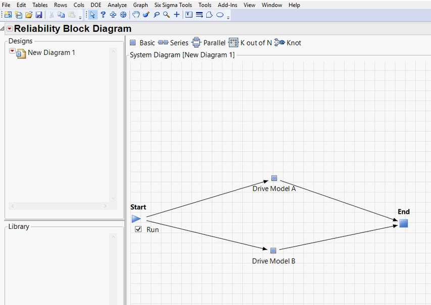
Connecting the drives in this manner is known as a “parallel” system and is represented in JMP Pro’s Reliability Block Diagram as shown below:

In this diagram, as we move from Start to End, there are “reliability paths” defined through each of the drive models. As long as there is an unbroken path from Start to End, the server works. So, if one drive fails, its path is broken…but there is a second path still unbroken through the second drive.

So the question becomes: what will the overall server reliability be with these two parallel drives? We know from the individual model analysis that Drive B should perform better than Drive A. Will the overall reliability be governed by Drive B or Drive A? Or will this configuration result in server reliability that is better than either of the drives by themselves?

It turns out that the server with the parallel drives will be better than either of the drives by themselves. In fact, the probability of server failure at any given time is the product of the failure probability of the individual drives at that time. As we showed above, Model A’s failure probability is 51% at 10K days, and Model B’s is 41%. Therefore, the server’s probability of failure at 10K days is 0.51*0.41=0.21. Restated, at 10,000 days, an estimated 21% of servers configured in this way will fail.

How can this be? How can the total server reliability be better than that of the individual parts?

Remember that we are talking about estimated reliability of a group of parts. Individual servers are made up of individual (i.e., unique serial number) drives. If a unique Drive A decides to fail early in its life, there is still an individual Drive B that could live beyond its average life. And with a very good individual Drive B, overall system reliability for this particular server will be better than the average failure rates shown earlier for the individual components. In a sense, Drive B has Drive A’s back. If you work through the math, you’ll see that it works!

A second example: Drives connected in series

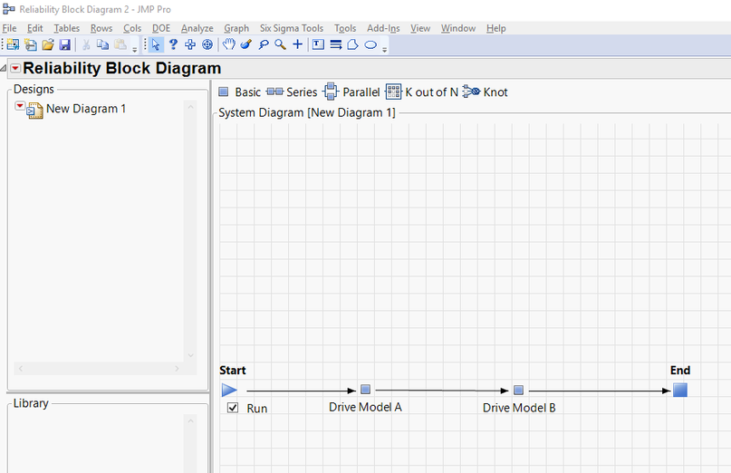
What if we could connect the drives in series? In other words, Drive A would have to be functional in order to pass information through Drive B, which would also have to be functional for the server to work. This series configuration is shown below:

In this case, the total system reliability is worse than either of the individual drives. Here is the equation for determining estimated probability of failure at any given time:

Plugging in the values of 0.51 and 0.41 for the failure estimates at 10K days for Model A and Model B drives, respectively, gives:

So, in this configuration, we would expect 71% of our servers to fail by 10,000 days! This is a much higher failure rate than the parallel configuration (21%) and higher than either of the individual drives alone.

Reliability Block Diagrams in JMP Pro

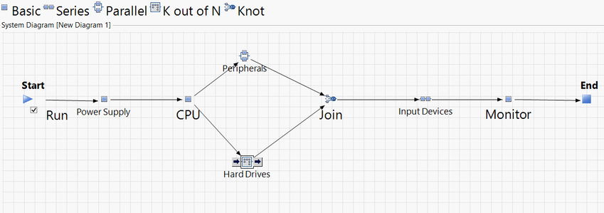
Of course, systems are always more complicated than those discussed above. For example, a more complete model for a computer system might look like this, with parallel and series connections:

An automobile braking system might be modeled as follows:

The good news is that you don’t have to work through these calculations on your own. JMP Pro does it for you. You can quickly make a system as complex as you like (combining parallel and series components, and applying many different failure distributions as your components dictate), and JMP Pro will estimate the system failure probabilities for you!

If you are interested learning more about Reliability Block Diagrams in JMP Pro and how they can help you in your work, watch this presentation by Dr. Bill Meeker..