Hello everyone.

Thank you for attending this experience sharing session on JMP.

My name is Stephane Georges,

I'm R&D Project Manager at Clecim, and I'm very keen on data science.

Today, we'll talk to you about the design of experiment methodology,

and more specifically, about the case we encountered when trying to find

optimal parameters for laser welding process.

During this presentation, I will show you how we use JMP for various platform

and how JMP adapted to the reality of the field by taking into account

a very irregular study area and a very imperfect study matter.

Without further delay, I will start my presentation

by telling you who we are and what we do.

Clecim is an engineering and production company of equipment

for the steel industry.

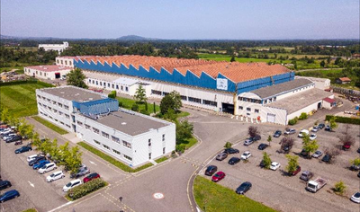
We are located in Montbrison in France in the surrounding of Lyon.

The history of Clecim is not new,

as we celebrated five years ago our 100th anniversary.

The area of the site is about 12 soccer field where work 230 employees,

mainly composed of managers and technicians.

A s we like statistics when working with JMP, here is the first one.

Our population is composed mainly of men, about 80 percent and 20 percent of women.

Concerning Clecim activities:

Our first activities is studies and consulting activities

for our flat steel producer customer.

We supply individual machine, or we supply a complete production line

such as pickling line, annealing line, galvanizing line, painting line and so on.

We also have an activity of services

for the furniture or spare parts, for export missions, maintenance,

and so on.

I put on this picture a typical layout of a galvanizing line.

This is to give you an idea of such processing line.

This one is dedicated to the automotive market

and the length of such an equipment is about half a kilometer,

so a very huge industrial plant.

When I talk previously about a machine,

I had in mind rolling equipment such as rolling mill, plate levellers,

automated strip surface inspection system, and even laser welding machine.

This is on this last equipment that we are going to focus on right now.

I will now talk to you about autogenous laser welding process.

Autogenous means without filling wire.

I will talk also about the parameter and factors that govern this process.

But first of all,

I would like to introduce our machine, the subject of our study.

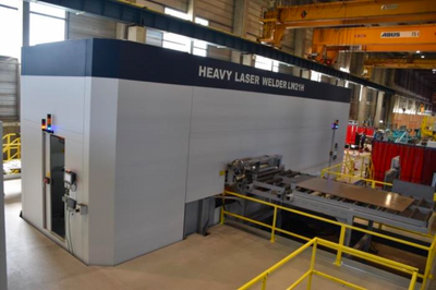
On the left part of the slide, you can see our welding machine.

In fact, not only our welding machine but it's containment,

the machine is inside the containment

for safety reasons because we are using laser.

The dimension here

of the door gives you an idea of this welding machine of scale one.

This is a huge industry, our welding machine.

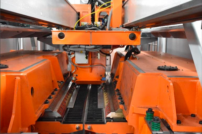
On the right part of this presentation, you can see a partial inside

of this welding machine, where you can see the clamps

and the [inaudible 00:04:37] of the machine.

Inside, you see the top portion of the strip,

the head and the tail of the strip,

that will be, first of all, cut also with laser and finally brought together

in order to be welded.

I will now talk to you about our target and constraint.

Of course,

our objective, our target is to have a good weld.

To do that, we need to achieve two objectives.

The first one is to have a weld seam which is defect- free.

Here on this slide, I put you an example of such a weld.

This is picture number one.

You can see on this picture that this whole thing is quite nice

without any defect.

When I talk about defect, here is a list of the typical defect

that we encounter when trying to weld with a laser.

Typically, we could have some patterns.

This is picture number two.

This is a top view.

In such a case, this is the molten material,

which is ejected from the top of the weld.

We could have also chain of pearls.

This is picture number three.

This time this is a bottom view,

and this is some droplets at the bottom of the weld seam.

We could have also

other defects, such as humpings, underfillings, or even holes.

This is picture number four here.

And here, typically, this is the case

when we have a very low travel speed and a very high power density.

Instead of welding, we are drilling at the material

and we create some holes.

Of course, this is we absolutely want to avoid.

Otherwise, we will decrease the resistance

of our weld.

This is a transition for the second objective

because we want not only the weld seam to be p erfect,

but we want it also to be resistant.

This is evaluated via an Erichsen type cupping test,

so this I will describe it a little bit later.

Our target is to have a trend as close as possible

to the one of the base material.

I will now talk to you about the last welding parameters,

the factor governing the process.

On this left part of this slide,

I put you a very schematic view of the process.

In gray at the bottom,

you can see the two pieces of material that we want to weld together

that can be of the same nature and thickness on it.

In yellow, this is laser welding head

that is connected in blue to its laser source.

In order to imagine

the kind of power that we use

for such an application, imagine that when you use a laser pointer,

typically for a presentation,

such kind of device has a power of just one milliwatt.

Here the last source we use has a power of 12 million times.

It is 12 million times more powerful that's such a small device.

Just to explain that we have a very huge power.

We need very little power to cut our material

and to weld also this material.

On the right part of this presentation,

I could use the process parameter, the typical process parameter,

which can be, first of all, the laser power,

the travel speed of the welding carriage,

the focusing distance, the gap between the plates,

the thermal treatment that we can apply afterwards, and so on.

But in fact,

for simplicity reason, in the rest of this presentation,

we will focus only on the two main one,

which is the laser power and the travel speed.

We will also consider

that the materials are identical and of the same thickness.

You will see that just with these two parameters we will have enough to do.

Okay, so the picture is set.

We have two targets.

One is to have a weld seam free of defect

and we want also to have its resistance.

We are now going to focus on our case study towards a good weld.

Our first target is to have a weld , which is defect- free.

We are going to search for what is called weldability lobe.

To do that, we need to get some data.

To get some data we will use the so called Power JMP procedure.

In that case, nothing to do with JMP, even if JMP is a powerful software.

But

this is how the procedure is called.

The picture on the bottom gives you an example of such a procedure.

At a fixed speed, we will perform 11 successive Power JMP.

In that case, we will switch from two kilowatts to eight kilowatts

to three kilowatts and so on.

The target is to reduce the number of options we have to do,

and in just one weld, we will have 11 sample

and we will have 11 observations to do.

Afterwards, we will visually examine

the upper part of our bead, the lower part of our bead

for each slot of this sample.

All of these data are collected into JMP

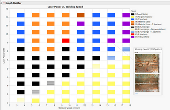
and we will use the Graph Builder platform in order

to display this map.

This is what I'm going to show you right now.

I go to my JMP journal here.

We will have four steps to follow.

This is our first step, building the welding format.

I will open

my table.

I collected all the data in this table.

I have all my parameters here, so the laser power, the welding speed.

In this column, I inserted my visual observation.

Is there any penetration? Yes/N o.

Do we have material loss? Yes/N o.

Humping? Yes/No, and so on.

A t the end of this file, I also put, as you can see,

I had two additional columns

of expression vector type where I have inserted

the picture of all my observations.

As you can see here also, I requested to have this information

displayed in the study area.

Now, we are ready to open our Graph Builder.

Here

I can learn it, okay?

All the data has been collected in this map.

Here you can see that on the X- axis, I put my welding speed.

On the Y- axis, I have my laser power.

I have associated for each defect color or shape.

A lso, we can have an association of the color and shape in that way,

which is a convenient way because we can overlay

four different type of defects at the same time for each point.

This is what I'm going to show you.

For instance, if I take this blue point here,

according to the legend, we have top spatters.

This is exactly what my pictures show you.

Here, this is the picture of the upper part of my weld,

here is a picture of the lower part of my weld.

Here we can see that we have effectively top spatters,

whereas the bottom part is defect- free.

For instance, if I take another one, if I take this purple one here.

So purple, this is the association of the blue defect and the red defect.

We have top spatters and bottom spatters,

which is effectively what we can see here on that picture.

This is a convenient way to see if effectively.

I have no mistake in order to know the magnitude of the defect.

This feature using the pictures is also very convenient because, for instance,

if I take this point here and I lock the pictures,

and if I take this additional point here and I lock also the pictures,

we can see that for constant laser power, I can compare the pictures

and see what are the effects when varying the welding speed.

In that case,

when we increase our welding speed, we can see that the width of our weld seam

decrease both on the top and both on the bottom.

This is a convenient way, let's say,

to dip into the understanding of our process.

I will close that.

I'll come back to my study case.

We are interested in the good weld area.

This is the area that I'm going to highlight here.

This is the black area.

Okay, like that.

Okay, this is our area of interest.

Now, what we want to do,

let's say, to investigate

the behavior of our weld seam

from the resistance point of view on that typical area.

Of course, we want to do it with a minimum number of tests

and we will perform a design of experiment

on this very

irregular study area.

Okay, so I go back to my presentation.

But

before answering into the conception of the design of experiment,

we have another interesting topic to do with JMP,

because we have, first of all, to study the strength of our base material.

We have to evaluate

the basic strength of the material via an Erichsen- type cupping test.

Why are we doing that?

We have three targets, three objectives.

The first one this is to establish

a reference from the strength point of view.

In that way, we will be able to compare

the resistance of our base material with the resistance of our weld seam.

This is the first point.

The second point is to be able to compare the two pieces of material

that our customer sends us.

We want to be sure that these two pieces

have the same behavior.

For that, we have to ensure

that they can be comparable.

The last point is that we want also to check that the plates are homogeneous

from the resistance point of view and that they do not present

any resistance profile in their widths or in their lengths.

To do our Eric hsen-type cupping test, we will do that on the base material.

This is what is mentioned,

what is highlighted here in the three first pictures.

We do not have any weld.

We're just performing this Erichsen- type cupping test.

For simplicity reason

I will call this procedure ball test in the remaining part of the presentation.

These three ball tests, we do them on three different positions

of the material, one located at the center of our sample,

one located on what we call the drive side on the machine,

and one located on the operator side of the machine.

For one sample, we do free tests.

What is a ball test?

In fact, this is explained

in the pictures located at the bottom of this slide.

We simply take

a bowl made in titanium, and we will press it from the bottom

and we will register the deformation of the material,

and we will register

the breakage force.

We do that for our two plates,

and we register all of that in JMP and analyze the results in JMP.

We will use the distribution platform and the Fit X by Y platform.

This is what I'm going to show you right now.

I go back to my JMP journal.

This is our second step, analyzes the base material.

I will open my file.

Here, I put all my data.

My plate ID, plate number 1 and 2.

For each plate I do that twice.

For each sample, we perform the measurements

at three different locations,

and here are the recorded value, the recorded strength.

We will analyze all of that and I store everything into a dashboard.

First of all, this is interesting to see visually our result.

I will focus, first of all, on this custom map shape.

In blue, you have the data for the first plate,

where I have my first sample and second sample.

For each sample, I have my free ball test, one located on the operator side,

one located in the center, and one located here on the drive side.

We have the same for the second piece of material.

What we can see here is that the resistance

goes through the following rates, so from nine to 10.4 tons.

Nothing really particular to see, except maybe that

here in the operator side, we can see that we have on the same side

the external value.

Here is the lowest value and here is the maximum value,

so maybe that will be something to look at

but we will come to this a little bit later.

Our target is to perform an ANOVA in order

to see if our two plates can be considered as comparable.

But before doing an ANOVA,

we need to ensure that our data follow a normal distribution

and that our variances can be considered as equal,

so this is what we are going to do right now.

Here are the distribution for plate number 1, for plate number 2.

Okay, I know that I do not have a lot of data,

but we will consider that we have enough to perform the test.

We will look at the two Anderson-Darling coefficients here.

What the p-value tells us is that we cannot reject the hypothesis

that the two plates can be comparable so that's good.

Then concerning the variances, so here we use another platform,

but we first go at the end, we perform the variance analysis here,

and we will look at the F Test, and the F Test tell us

that we can consider as our variance are equal.

As our data are normally distributed on our variant article,

we can apply safely our ANOVA.

This is what is mentioned here.

On the top part, you have the drawing.

Here are the associated data.

I will not focus on the data.

We will just have a look at the pictures.

Here, what we can see,

this is the extremities of the two diamonds overlap.

We cannot reject the hypothesis that our two plates are different,

so this is good.

We will now reach the conclusion that our two plates are equivalent.

We can now aggregate all the data.

This is what is done here in the distribution.

We put all our data together,

and finally, we have a global resistance of our plate of 9.76 tons

plus or minus 0.17 at two standard deviations.

This is the first point and we will use this information a little bit later.

Another interesting thing,

so this is what is mentioned here.

We can also perform the ANOVA taking into account the position.

And this as we have previously observed,

we can see that the run variation on the operator side

is a little bit higher

compared to the drive side and the center of our plate.

We want to understand a little bit why such things happen.

To do that, I will come back to my presentation,

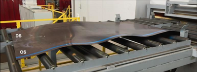
we will have a look at the plate.

We are studying at the moment.

Here is the appearance of our sheet metal.

What we can see is that on the drive side here,

our plate is nearly flat, I would say.

But on the contrary,

on the operator side, we clearly see that the plates have some waves.

I do not know exactly what is the history

of this material, but we can clearly imagine that

there was a trouble at the rolling m ill or the plate leveller

and that the higher force has been applied on the operator side,

leading to this kind of periodic modification of the resistance.

This is a new constraint because we have to take into account

this new information in our design of experiment.

I will sum up all the information we have before building our design of experiment.

First of all, I remind you that we have a very irregular study area.

This is a black area that is mentioned here

in the drawing.

The traditional way

to deal with such things in JMP would be to fill up a linear constraint.

But here due to the shape of this area, it's a little bit difficult.

Instead, we prefer to use the Candidate Points technique,

which is called also Covariates engine.

I remind you also that we have an inhomogeneous plate

and to deal with this phenomenon, we will have to introduce a few parameters

into our design of experiment.

First of all, we have to take into account the strength variation in the width.

To do that, we will introduce a categor ial parameter,

a 3 levels- categorial parameters,

and the three levels are drive side, center, and operator sides.

In order to deal with the periodic variation of the resistance

along the length of the plate, well, this is a little bit difficult,

because, in fact, we do not control this parameter.

We have to be on

this variation.

For that, we will introduce the weld position

from the head of the plate, or in millimeter,

and we will introduce it as an uncontrolled parameter.

Finally, this is not finished.

This is what you can realize, what you can see

in the last picture at the bottom.

This is typically here a picture of a weld,

where are located above three ball tests.

Well, these ball tests are not independent.

They belong to the same treatment.

They belong to the same weld.

They are at the same weld position.

We are

in the presence of split/ plot design,

where we have hard and easy- to- change parameter.

This is a lot of constraints we have to take into account.

Now, I will show you how to do that with JMP.

I can go back to my JMP journal, so this is our first step.

But I will show you from the beginning and I will go back here

to this step.

I come back to the file I had previously.

I will select here

all the rows with a Good Weld.

I will also select

another power column, my welding speed column.

In the table here, I will extract a subset of this table.

I will extract selected line.

I will extract the selected column here.

Okay, I will build my subset of Candidate Points.

But here is the tricky thing because, in fact,

as we have a design also, I need to tell them that

you will have the possibility to select three times each point.

I will multiply by three this number of points.

There is probably a lot of way to do that.

In my case, I will just create three columns,

one call it drive side,

one call it center,

one call it operator side,

and I will just stack all these

using that three columns.

Here I have created my set of Candidate Points.

With the Graph Builder, I will check that everything is okay.

In the Y- axis, I will put the laser power. On the X- axis, I will put the laser speed.

Here, we can recognize the shape of our irregular study area.

I will also put here the label into the color sections.

Each of my points has been multiplied by three.

This is exactly what I wanted.

I can use this as a starting point.

This is a set of my Candidate Points.

I could have additional points.

I could have done a little bit all of that.

I could have added some points here, for instance, and so on.

But to be honest, the discretization steps are fine for me.

I will keep all the points like that.

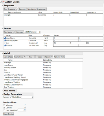
I will open now my design of experiment menu,

go to my Custom Design platform.

In the response, I want to measure the strength of the material.

In the Factors, I will add my first parameter,

Laser power and welding speed as Covariate.

I select Covariate, I select laser power and Welding parameter.

Automatically, JMP fills up the lowest and highest value for these two parameter.

I will add also my 3-level categorial parameter.

I call it side,

and my level drive side,

center, and operator side.

I do not forget also to add my uncontrolled parameter.

This is the position of the weld.

This is an uncontrolled parameter.

I do not know the limits, so I put nothing in these boxes.

I also do not forget to change here

in order to take it into account the speed/plot feature.

I mentioned here that my laser power and welding speed are hard-to-change

compared to the side.

Everything is correct here, so we can run.

Concerning the constraints, I do not need this area,

because I already took into account my constraints

when selected my covariate, so I do not need here.

Concerning the model, I immediately choose RSM.

But in that RSM, I will suppress the interaction of the laser power

with the position and the interaction of the position

with the welding speed

because there is clearly no interaction at all.

I will immediately click on the Make Design button

because it will take some moment.

Here we can see that JMP proposed me

to perform eight tests with 24 measurements.

This is fine for me.

I keep this default parameter.

I make my table here.

Okay.

This is the defect concerning to laser power, welding speed, side.

I have the column ,

I will record the position of my welding speed,

where I will record the strength, so everything is okay.

I will never visualize the point into the Graph Builder.

I put, once again, the laser power in the Y- axis,

the welding speed will in the X -axis.

Perfect, and we read curve.

I will also put the side here into the Color area.

I will add some details.

Okay, here we can see that this is the point

that has been selected by JMP within the framework of our Candidate set.

For each point, I have to perform three measurements,

on drive side, center, and operator side,

and JMP wants me to perform this test twice.

Okay , so this is what we have done.

I will now show you the result.

I go back to my JMP journal here.

This is our last step, the result analysis.

I will open the associated table.

Here, this is the same table as previously.

I have recorded the positions.

I have recorded the strength in absolute value in terms.

I have inserted two columns here.

This is our

reference strength,

the strength of our base material that we have previously determined.

This is 9.76 tons,

because, in fact, I will use it in order to create this extra column,

this is the strength, but in percent compared to the base material.

This is on this last column.

This is the first column that we will take into account in our optimizations.

I store my analysis into each column here.

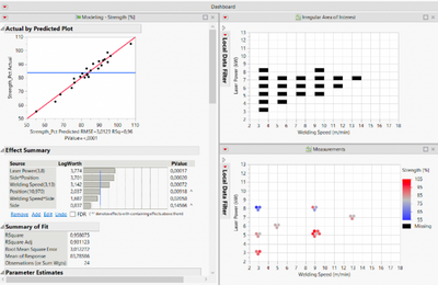
Here are the results.

As a reminder, I put on the right part.

the irregular area as a reminder.

Here are the experimental points that we have performed.

I have colored the point using the strengths in percent.

I use the Fit Model platform in order to create my model.

Step by step, I have suppressed the non-significant interaction

of our parameter

using the p-values here.

Finally, I have a model

with an explicative power of two of 96 percent,

which is quite good because, in fact, it means

that only four percent of the wall variation

escape to our prediction power.

Concerning the collinearities , if I look to our VIF,

our variance inflation factor, all of them are below three.

We can be now confident

in our model and we can use it in prediction.

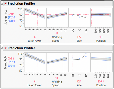
We can go to the prediction profiler here.

First of all, I will focus on this part,

on the interaction of the position with the side.

What you can see here,

if I move the position of the weld,

it seems that the resistance is not sensitive

to the positions on the drive side and center.

But on the contrary, on the operator side, this one is clearly

influenced by the positions.

This is exactly what we have seen in our plate.

This is a modeling of our waves.

Here we do not see this kind of shape because this can be easily explained.

Our weld are not so huge.

It's only a sample of six centimeters.

We do not consume a lot of material.

We do not go along the wall

with that shape.

We go from the bottom to the top only.

We are quite happy because we were able

to analyze and to model correctly this behavior.

This is interesting because

we can now have access to the pure effect of the laser power and welding speed.

This is what is mentioned here.

For this particular material,

we can conclude that we can increase the resistance of this material

by decreasing the laser power or by increasing the welding speed.

Now what we have to do

this is to determine an optimal point using all the information we have.

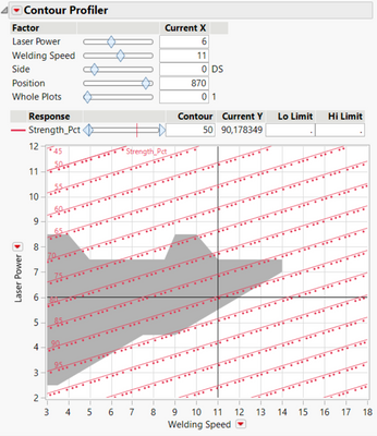
To do that, we prefer to do it using the control profiler.

This is what I have mentioned here.

In this control profiler, once again, I put in the X- axis,

the welding speed, in the Y- axis, I have the laser power.

I have reproduced

my area, my irregular area

where I am defect- free.

To do that,

I have simply

implement a script.

Here is a list of points,

and I just asked JMP to use this point and to draw a polygon.

I have my black area where I am defect- free.

On that drawing, I have also inserted the ISO resistance curve.

Here in red, you can see the values of this ISO resistance.

We can see that, here, we go from 50 percent to nearly 100 percent.

Before doing the optimization, I will add another constraint.

It's not enough.

From the productivity point of view,

we want, of course, to go as fast as possible and we want to have

the highest welding speed.

Using all that information, we have selected

the point at six kilowatts and 11 meters per minute.

This is the point that has been located here.

Why?

Because this point is located in the black area,

where the w eld seam is free of defect.

We can see using our model that we expect this point

to have at least a resistance of 90 percent of the resistance

of the best material.

What is interesting also is at this point

we have enough safety merging around this point.

Of course, we have tested this point and this is the result.

But I'm going to show you right now.

I go back to my presentation, which is located here.

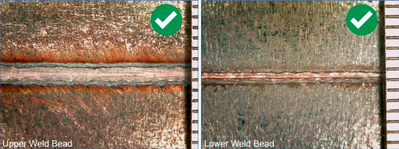
This is the result of the optimal point we are choosing.

First of all, on this slide, you can see on the left part,

the upper w eld bead pictures,

on the right side, the lower weld bead pictures.

You can see that the weld seam are free of defect.

We have no patterns, we have no droplet, no chain of pearl, no holes, et cetera.

This is what we wanted.

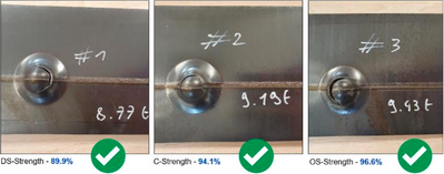
From a resistance point of view, first of all, if we focus on the pictures,

we can see that this is the material that breaks

and this is not the weld seam that opens, so this is the first good point.

Concerning the resistance, we can see that each of them

are higher than 90 percent.

This is exactly what we wanted,

let's say that we have achieved our target.

This is the end of this presentation. This is now time to conclude.

First of all, I go back to my JMP journal, I would like to mention that

with this presentation, you have the possibility to download an article

that will be located

on the website.

Here you have a full article explaining all the case studies.

I have added additional material.

If you are interested in knowing more, please feel free to download it.

A s a conclusion, I would like to mention

that if some of you are interested in knowing more about covariates,

I would like to mention two available sources.

The first one is an article that you can find

on the JMP user community

entitled

"What is a covariate in design of experiments?"

Also from the same offer,

you have a webinar entitled "H andling Covariates E ffectively

when Designing Experiments."

To conclude, I put here a quote from Mark Twain

that humorously tells us that

"Facts are stubborn things, but statistics are pliable"

Inspired by Mark Twain,

I would like to say that facts are certainly stubborn things,

meaning complex, but don't panic

because, in fact, JMP can easily adapt to the reality of the field.

In my case,

he was able to adapt to a very irregular study area

and also to a very imperfect study material.

This is the end of my presentation.

I will now answer your question, so please feel free to ask.

If we run out of time, I mentioned here my contact information,

so please feel free to contact me,

and so I'm waiting now for your question.

Thanks a lot. Bye bye.