
My name is Per Vase from NNE, and I will together with my colleague Louie Meyer
represent how you can use JMP in pharma process validation,
and actually leading into that you can do
continuous process verification afterwards.
We both come from a company called NNE, and we do consultancy
for the pharmaceutical industry and we work with data science.
So we actually trying to create value from data at our customers.
Of course, we are extremely happy that we can use JMP for that
and this is what we are going to demonstrate today.
So the background for the presentation is process validation.
This is a very important issue in the pharmaceutical industry,
that before you launch a new product,
you have to prove that you are capable of producing it.
Classically this has been done by just making three batches.
If these three batches were okay, we have proved that we can manufacture
consistently and then you're ready to launch products.
But of course everyone,
including the [inaudible 00:01:06] have found out,
that you could make three batches is not the same,
as all future batches are going to be good.
What is expected today from a validation is that not only show that you can make
three or could make three batches,
you're suppossed to make a set of batches.
Based on this set of batches, you should be able to prove
with confidence that all future batches will be good.
So instead of predicting the past, we now have to predict the future.
This really something that is a challenging thing in the pharma industry
because they have been used for many years just to make these three batches.
So how to do it now?
We are really helping many customers with this,
and what we strongly recommend is simply predict the future.
How can you predict the future?
Well, you can do that in JMP with prediction intervals.
That's what they are for.
So you collect some data, on the days you analyze,
you can predict how the rest would look like.
If you can just build a model that can describe your validation data set,
and if you put your batchess in this model as a random factor,
these prediction limits actually cover not only the batches you make,
but also the batches you haven't made yet,
and thereby you can predict the future.
What you're seeing in the bottom of the graph you have stage one.
This is where you designed the new process for making the new product.
Stage 2 is exam that's the classical old fashioned validation.
Where we previously made three batches, now we are making a set of batches.
Now based on that we will predict the future batches will be good.
If you have a lot of batch to batch variation,
it can be hard to predict with just a few batches,
due to the width of the T distribution which view the use of freedom,
so it might take more than three.
But we strongly recommend still to make trees stage 2 because otherwise,
patients have to wait too long for the new product and then if it's not enough.
You can make the waste in what we call stage 3a.
Certain parties that treat hopefully on how your prediction limits
will be inside specification limits and then you have proven
that all future paths will be good, and you can go into what we call stage 3b,
meaning that now you don't have to measure in product testing any longer.
You could maybe measure on the process instead of measuring on the product
because you have proved all future medicine will be good.
You only have to prove that you can maintain the validated state.
That can give you a heavy reduction in your future costs.
Some customers, they get you up to 70% reductions, in the future costs,
after they have proved that all future batches are going to be good.
Today we will try to demonstrate, how this can easily be done in JMP.
So what is the validation all about?
Well, it's the prediction of future batches.
Now, previously we just made three batches,
but now we have to predict the future batches.
How can you predict that with confidence?
Because when you do validation you have to prove confidence, things are fine.
Well, you can just use prediction intervals.
They're also called individual confidence intervals and JMP for the same reason.
Or you can also go for tolerances, if you want.
How many batches in stage 2?
We actually recommend to go on with what they used to, which is three.
But you can only pass with the three batches if you control limits.
Control limits are actually just predicting limits without confidence.
I will show you how to calculate them, and if they are inside.
Actually the best guess it's fine.
If your predictions are outside, you might need more batches.
But you can make these after have gone to the market with your product.
How many batches should they make in 3a?
Very simple.
Until your prediction limits are inside specification intervals.
Or if you want, the corresponding PPK is high enough.
I will show how you can convert these limits to a PPK.
When it's passed you can actually go to stage 3b because now we have proved
all the future batches will be good.
You just have to prove that you can maintain the validated state.
Typically that can be done by measuring in the process,
which is easier in real- time, compared to doing in product testing.
So that's actually a huge benefit.
A lot of people harvest if you're doing it this way.
That's a small flow chart for how does it work.
So you start out looking at your validation once,
you calculate your prediction limits,
just be aware that until version 15 they were not right.
They agreed to freedom two low prediction limits.
It was settled in version 16, so please JMP use version 16 for this.
Then if these prediction limits are inside spec limit,
you have passed both stage 2 and 3a,
and you're waiting for continuous process verification,
measuring on the process instead of measuring on the product.
If it turns out that the prediction limits are too wide,
then look at your control limits.
If they are within spec limits, and predicted limits outside,
the most common typical course is to just collect data,
you just collect more data.
But you do that instead 3a after going on to the market.
So just recalculate this prediction limit, every time you have a new batch,
and then hopefully after maybe three or four extra batches,
they are inside your spec limit and then you're ready to go.
If it happens that also your control limits are outside specification,
then actually you're not ready for validation because then actually
best guess is that the process is not capable,
and of course you have failed your validation and you need to improve
the process and we do everything again.
Hopefully we don't end there.
But of course it can happen.
Just short about this particular methods
we have used to calculate these control limits,
prediction limits and tolerance limits.
For control limits,
you need the JMP of course, you can get control limits.
But it's actually just for one known mean and one known standard reason.
Often you have more complex systems that you might have many means,
different cavities and decent moving process for example,
you might have several bands components between sampling points.
Typically you have more than one mean and one standard reason.
But then you can just build a model, and describe your data set with the model.
Then you can just take the prediction formula,
you can send the standard error or prediction formula
and you can take your standard error on residuals,
and then instead of multiplying with the G quantile,
just use the normal quantile.
Then it corresponds to having back confidence.
This is how we calculate control limits based on a model.
Simply based on the prediction formula and the standard of the prediction,
the standard of residuals which we can all get from JMP,
then it's pretty easy to calculate how does control limits work.
It's even easier to predict the limits, because they are ready to go and JMP.
They're already there,
and of course they would just use the limits calculated by JMP.
I said before be careful with JMP.
Before version 16, limits simply gets too wide.
So please use version 16 and newer for this.
For tolerance limits,
we have a little bit of the same issue as with the control limits.
You have tolerance limits in JMP, but only for one mean,
and one standard deviation.
We don't have it for a model.
But it's actually pretty easy to convert the classical formula,
for a tolerance interval into taking a model.
Just replace the mean with the prediction formula.
Just replace N minus one with the degrees of region for the total variation,
which we actually calculate from the width of the prediction interval.
Then you can just enter this in the classical formula and suddenly,
we actually also have a tolerance interval and JMP,
that can happen within and between batch variation.
Then we ready to go with the mathematics here.
Some customers prefer not just to look at if limits are inside specification,
they need to be deep inside specification,
actually corresponding to that PPK is bigger than one.
But it's very easy to take the limits and the prediction formula,
and convert them into a PPK by this classical formula for PPK.
If you predict the limits, you get it with confidence,
because the average confidence the same retirement limit,
and if you put it in the control limit, you just get PPK without confidence.
We'll do without confidence and with confidence.
Without confidence is the one we supposed to recommend to use in stage 2,
and the other ones are clearly for stage 3a,
where we have to prove it with confidence.
So life is easy when you have JMP,
and if you have a model that can describe your validation dataset.
But we have to be aware that behind all models,
there are some assumptions that need to be fulfilled,
at least to be justified before you can rely on your model.
You need to do a standard check of your data,
before you can use the model to calculate limits.
A s you know, JMP has very good possibilities for this,
and I will just now go into JMP, and see how this works.
Here is a very well-known data set in the pharma industry,
published by Industrial Society of Pharmaceutical Engineering,
where they put out a data set from the real world and say,
"This is a typical validation set, please try to calculate on this and see
how would you evaluate this as a process validation data set."
If you start looking at the data chart, you can see here we have three batches.
The classical three batches, oldfashioned ways,
and we are making tablets here and we are blending the powder.
When we are blending the powder, we take out samples in 15 different
systematic positions in the blender in all three batches.
When we take samples, we take more than one.
We actually take four.
So we have three batches, 15 indications, and every time we take four.
This is a data set from real life that was used for validation.
If you look at data,
it's actually fairly easy to see that for batch B within a location,
the inter batch's location evaluation is much bigger than for batches A and C,
and if you put a control limit on your standard deviation,
that's clearly C is higher.
You can also do heterogeneity of variance test.
It will also be fairly obvious that B has significant bigger variance than A and C.
So we cannot just pull this because you're only supposed to pull variances,
that can be assumed the same.
So what to do here?
Well, the great thing about JMP,
you can just do a balance model, so you can go in and put in the batches
as a balance factor on top of having factors to predict the mean.
A gain you can clearly see that patch B,
has bigger variance than A and B and we need to correct for that.
So how do you correct for that in a model?
Because I would like now to put in random factors
but not where its modelled in JMP do not support random factors.
What I do instead, I just go up here and I save my variance formula.
So actually I get a column here, where I have my data variances.
Then I can just do weighted questions with inverse variance.
Classical way of weighing when you're doing linear regression.
So it's very easy to correct for that patch B has higher variance
than A and C, just by doing weighted regression
Being aware of that, then I can start looking do I need to transform a data?
You know you have back drops and information and JMP.
So it's very easy,
just make an ID that describes the combination of batches and location.
Then you can look at the procedure variation within each group,
and pull this across, and you will get a model like this.
You can see I weighted it because I had to weight it.
To correct for batch B as I have in A and C.
You can then see you have no outliers and you can also box -cox.
There's no need for transformation.
So that's also easily justified working this way.
Then I'm ready to make my model.
But when I make my model, I will put in my batch as a random factor.
I might also put in location times batch as a random factor,
because it should be random because I would like to predict future batches.
Then there's actually another assumption,
because when you put in random factors you are assuming the influence
at least on average zero and it's normally distributed.
How to verify this or justify this?
Well just go and look at BLUPs, that's just a random factor.
You can just make them into a data table, and you can do a BLUP test on them.
That's what I have here.
Here you can see I have saved my batches' BLUPs and my interaction BLUPs,
and I just re -modelled them to these.
I can see these batch effects can easily be assumed normally distributed
and actually the same with the interaction effects.
Now in a very short time, all the sensitive check you need,
to be able to justify that you are ready for analysis.
So now I have my model, which I'm ready to go for,
where I have put in my locations in the random factors,
and my pass as my other factors.
Now I will give my work to Louie,
who will now show how to go on with the script on this data file.
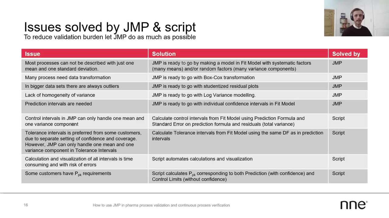
As Per's already shown,
JMP already offers a lot of opportunities to deal with many of the problems
you're facing and validating, for example, TPQ batches.
Some of the things he has shown here is that,
in fact most processes cannot be described by just one
mean and one standard deviation.
For this we really like the state model platform,
which allows us to do exactly this by including system manufacturers for many
means and or random factors for many variances.
Then often we see the data requires transformation.
Here we already the fit model platform has the box- cox transformation allowing this.
Furthermore, data sets almost always contain some kind of outliers.
For this we are already in the midmarket platform,
also have the student type residual plus,
which is a great way of dealing with outliers.
Then in cases where we see a lack of variance from beginners,
JMP has also the log variance modelling, which we use to find the variance,
and convert it into a weight in a recursion model.
Then out- of- the- box JMP of course also have the prediction intervals,
individual confidence intervals directly from the Fit model.
There are also some of the problems we faced where JMP didn't take us all
the way but did the groundwork here.
I think this is what we're actually trying
to address with our script as well, making it much easier,
and I think one of the primary reasons we
have developed this script is that usually the customers we see that these
calculations and visualizations we're doing often are done by human employees.
So whenever humans are involved,
there is a high risk of human errors as well.
This is what we are trying to battle by automating all of these steps later
on coming from the analysis and also the visualizations.
Then of course, here is the control intervals in JMP,
where JMP can only handle one mean and one variance component.
This will also solve in the script
from the fit and model platform using the prediction folder instead of the mean.
Then we use the total variance
from the model calculated from the standard error and the prediction
formula and the standard error on the residuals.
Then we also often face customers who prefer tolerance interval issues,
and this is due to their separate settings of both confidence and courage.
However briefly described,
JMP can only handle one mean and one variance component tolerance intervals.
So in the script we also calculate
tolerance intervals from the Fit model platform using the same number
of effective degrees of freedom as used in our prediction itself.
And then lastly,
the script has also included the calculation of capability values,
more specifically the PDK values, as many customers also require these.
Here we calculate them both
with confidence using the prediction limits as an input to the calculation.
Then we also calculated our confidence using the controller input calculations.
So just to go to the script.
Our script here,
as we have developed package most of these subsequent steps, after doing the sentence
check into a single package, the script itself takes three inputs.
We have the original data file,
and then we have the model window and then we have a template document.
So what our script does is that it actually feeds information from the data
file and the modern window, into the template documents.
From the data file we take the metadata and data itself, and from the model window
we take model parameters and model results and fields as well.
This is also why it's important to stress here that the model
that are used here as an input should be a complete done model.
This means that you have done already
all the sanity checks SPI just introduced us to.
Also you have done your model deduction and the sanity check includes something
like outlier exclusion and data transformations as well.
One could argue that we could do this in the script as well,
obeying some hardcore statistical rules.
But we also think that this is a very useful experience.
Working with the model here.
You get a much better insight into the data,
and you also have to apply some process knowledge here to get a better model.
So the template document in itself,
we actually use this inspired by the app functionality and JMP.
We really like some script where the users
or each users can actually interact with the script itself.
So the template document is essentially
a data table in JMP where we have no data in it.
However, we have defined a lot of columns
with predefined formulas referencing each other.
This allows the user to actually go in,
and backtrack all our calculations through the columns in this template file,
leveraging the for example, formula editor and JMP,
and potentially add new columns if they want to see new calculations.
Or they can edit some of the calculations we are doing in there as well.
Furthermore, all visualizations descriptors providing the user
are also actually stored as a table script in the template document.
So users can just go in here and edit, for example, the layout of specific graphs
if they want new colors or something like this.
I think we should take a look at how it actually looks in reality.
We will jump into JMP here and I will just find the same model
as Per just finished for us.
We are again looking at the ISPE case as Pierre showed,
and I will just find the same model he ended up with here.
Now that we have our model, we have done the sanity check and everything,
we have our original data file behind, we simply run the scripts.
And we will need to send it to three things here.
First of all, we have template files now filled with all the data we need.
We see the two graphs we're showing right here.
Then we have the PPK batch giving us a PPK for each location in the blender.
We have a total of 15 up here,
and we have the normal PPK based on control limits in blue,
based on prediction limits in red and based on tolerance limits in green.
Lastly we had the graph here.
This graph shows us partly our data,
along with all the limits we have calculated in the script.
Yes, and what we see here is in fact that batch A and batch C
are performing well for all locations.
Meaning it has its prediction limits, and tolerance limits, and control limits
for that matter inside the specification for all locations.
However,
if we look at batch B,
where they also found the variance to be much larger than
the two other batches, we see that this is in fact going outside
specifications on all locations when we look at the prediction limits,
not necessarily both specifications, but either under lower and upper.
So we see many customers here actually just computing some average limits,
across A, B and C.
But we don't see that as an opportunity here because for us this tells us that,
if future batches behave like batch A or C, we are okay.
We can consider and say that future or observations of future batches,
will fall inside specifications.
However, the future batches behave like batch B,
and we cannot guarantee that we will have
all observations of future batches falling inside the specification limits here.
I think I would just also use this time to go through an example where we actually
also take into consideration the whole approach and that showed the flowchart,
and how we would actually do a PPQ validation using the script.
We've brought a customer example here, just find it here,
and this is affecting customers who have been through PPQ with the validation
and they have now produced all the batches.
So we will just quickly use a local data
filter to just look at the three first batches they produced in stage 2.
Here we have our model, and we run the script.
What we see here is that we find ourselves in a situation where we have
both prediction limits and tolerate limits outside big.
In fact they are quite far outside.
But the best guess determined by the control limit is in fact,
that we are inside specification.
So what this tells us is that we actually feel safe enough,
concluding that we have passed stage 2, and can now go into stage 3a.
Actually enable us by the customer to put their products on the market.
It's important to stress here that even though we go from stage 2 to stage 3a,
we do not reduce the [inaudible 00:23:22], and the production you see we have.
We are still fairly certain or really certain actually that,
no bad products should enter the market.
So what the customer would do next then, is simply to produce the next batch,
which would be batch four here included in the model, and then we run it again.
Of course you will have to do the sanity check of the model again,
including the new data.
What we see here now including the fouth badge,
is that we are in fact in the same situation as before.
However, both the tolerance limits, and the prediction limits,
are moving much closer to the control limit,
and even more important, they are moving towards the spec,
which is what we really want to see in this situation.
The reason this is that we actually noted within batch variation very well.
However, due to having only three or four batches,
we don't know the twin batch variation that will...
This is what actually gives us these four limits.
This would be an iterative approach, producing one batch, analyzing the results
and continues going on until you actually find the limits inside.
Now just include the two last batches, run it again.
What we see now actually is that we have all our limits inside specification.
This tells us that we now have passed stage 3a,
and we can now work towards reducing our heavy in productivity,
by implementing sampling instead of 100% inspection,
and continuous process verification and so forth.
This we're still having had our products on the market,
since the first three batches we produced.
In an image like the graph shown here,
you could be concerned that your prediction limits are this broad still.
The charterment limits are very close to spec.
So if you just go back to the situation where we have three batches,
one question here could be, "Are we actually safe,
when we have this broad prediction limits?"
Could we end up sending bad products to the market?
Here there are two very important points.
First of all, at this stage, we still have a very heavy unit in product QC.
They will ensure bad products does not go to the market.
Furthermore, we have to remember here that we are actually not trying to say
something about the specific batches we produced.
We are trying to say something about future batches.
If we want to assess the performance of these individual batches per batch,
what we actually have to do is that we have to go back to our model.
We go to the model dialog here, and we do not include batch as a random and fit.
We use this as a fixed vacant environment instead.
I'll just apply the local data filter,
and then if we run the script like this,
we will actually see how well we know the individual batches here.
Here we see, compared to the other graph, which I will just try to put up here,
we now have much, much narrower limits for each bad batch,
telling us that we don't have to fear that any observations within either
of these batches are actually outside specifications.
So it's the combination of this, and the heavy in product QC,
which actually makes us confident that we can have the three batches,
go to the market with the products,
as long as our control limits are still within specifications.
Yes.
So just to conclude on this, I will go here.
So, what we have been looking at here is how can we validate,
how can the inner validation use JMP to predict the future batches will be okay?
So we have seen here that,
if you can describe your validation data set with a model,
you can actually predict the future with confidence.
This can be done either by using the prediction intervals,
or the tolerance intervals.
So what we have made here and over here, is a script,
that actually automates visualizations of prediction intervals
and also the PDK values.
It calculates and visualize tolerance intervals using the same number
of effective degrees of freedom as seen when calculating the prediction intervals.
Then it also calculates and visualize the control limits.
But it is important to remember before using the script,
you have to go through the sentence the check is represented.
But here JMP already offers a lot
of unique possibilities to justify our assumptions behind the model.
This includes variance heterogeneity.
So if variances are not equal between the batches as we saw here,
we can use the log variance model to find a weight factor,
and through this weight factor, I made a weighted progression model instead.
We can ensure that our residuals are normally distributed,
and if they' re not, we can use the box-cox transformation to transform our data.
We can, through the Fit model platform also evaluate potentially outliers
through the student plug.
If there are any outliers,
we always exclude this from the model itself.
Then at last we can actually justify whether or not our random factors
are normally distributed through the BLUP test.
A gain, if we find a level here which does not match,
we will ask for the outliers and the studentized residual,
exclude these from the model as well.
You.
