- JMP User Community
- :
- JMP Discovery Summit Series
- :
- Past Discovery Summits
- :
- Discovery Summit 2014 Presentations
- :
- Using JMP® to Analyze Data From a Designed Experiment With Some Responses Below ...

- Subscribe to RSS Feed
- Mark as New
- Mark as Read
- Bookmark
- Subscribe
- Printer Friendly Page
- Report Inappropriate Content
Authors
William D. Kappele, President, Objective Experiments
Julie Kidd, Materials Engineer, US Synthetic
Heather Schaefer, Materials Engineer, US Synthetic
Introduction
Sometimes you come across an interesting problem in the course of your normal work. That's what happened to us. While using a designed experiment to formulate synthetic diamonds, we had a few trials we could not measure a response for – they were below the detection limit of our measurement system.
We could have changed the factor settings until we could make a measurement, but we didn't want to add that expense if we didn't have to.
At first we simply assigned “zero” to everything we couldn't measure. We were a little nervous about this though – after all, we were lying to JMP – something we don't like to do!
It is with the desire for honesty that our adventure began.
The Adventure
Two of our responses were below the detection limit of our measurement system. All we knew of these responses was that they were somewhere in a range between the detection limit and zero. Data that are only known to lie in a range are called “censored data.” We knew about dealing with censored data in Reliability Analysis, but we didn't know how to deal with it in a designed experiment.
We asked Bill if he knew what to do. He suggested we use Maximum Likelihood Estimation – but he wasn't sure how to do this in JMP. He contacted Brad Jones (of JMP) and Brad steered him to the Parametric Survival platform. While it wasn't designed to do exactly what we needed, it could be used to get our answer.
We wanted to share what we had learned – how the different analyses compared and how to use JMP to perform them – but our project was proprietary. It looked like our learning would have to be our secret until Heather came up with a great idea: disguise our work as if we were baking chocolate chip cookies! She and Julie then successfully created a “cookie” data set true to our work that would reveal no secrets.
As with all analogies, our cookie analogy will seem a little contrived. However, if you bear with us, you will be able to see the problem we really faced and learn how to deal with this same type of problem if it crops up in your work.
A Simple Analogy: Baking Cookies
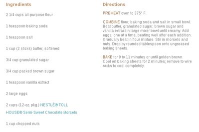
Suppose we were actually working on baking chocolate chip cookies. Our goal would be to produce the thinnest cookie we could using our recipe. (We told you it might seem a little contrived! We would really have been trying for thick cookies.) The recipe we used was the classic Nestle Toll House cookie recipe in Figure 1.
|
Figure 1 – The official Toll House Cookie recipe, courtesy of Nestle. |
We grouped the ingredients in a logical way to create 5 factors for our experiment. The factors are listed in Figure 2.
Chips Dry (flour, baking soda, salt) Creamed (butter, sugar, brown sugar, vanilla) Temperature Time |
Figure 2 – The factors. |
Here are the factors and levels we used to create our experiment design:
Factor | Type | Low Level | High Level |
|---|---|---|---|
Chips | Mixture | 0 | 0.5 |
Creamed | Mixture | 0 | 0.5 |
Dry | Mixture | 0 | 0.8 |
Temperature | Continuous | 375 | 450 |
Time | Continuous | 5 | 12 |
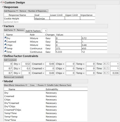
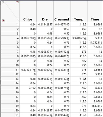
We also had several constraints. A portion of an experiment design with these constraints (see Figure 3) is shown in Figure 4.
Figure 3 – Creating the Design with Constraints |
Figure 4 – A portion of our experiment design. |
Then we baked cookies ….
Using JMP to Analyze the Data
After we baked our cookies, we needed to measure the thickness. Wouldn't you know it! We didn't have a very good ruler. We really couldn't measure anything under 1 mm. We could certainly tell that we had a thin cookie, but we couldn't tell exactly how thin. Our detection limit was 1 mm.
Initially we simply entered a “zero” for the thickness of cookies we couldn't measure – those below our detection limit. Remember, we knew we had a cookie, so “zero” couldn't have been right, but we thought we'd give it a try.
These data were easy to analyze. We simply used the “Fit Model” command with the “Standard Least Squares” personality.
In order to understand how we analyzed the data as censored, we need a little background.
Maximum Likelihood Estimation
While Least Squares is an excellent technique for fitting data to models, it isn't easy to use with censored data. Another technique, Maximum Likelihood Estimation, is much easier to use with censored data. JMP uses Maximum Likelihood Estimation at various times in the “Fit Model” command (for instance, if you choose the “Generalized Linear Models” option), however it only offers an option for censored data in the Parametric Survival platform.
We needed to “coax” JMP into doing what we wanted it to do.
The Parametric Survival Platform
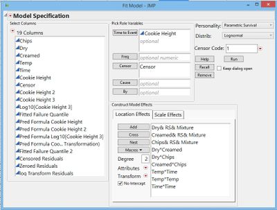
JMP's “Parametric Survival” platform uses Maximum Likelihood Estimation and offers the ability to analyze censored data. It is designed to work with “Time to Failure” responses – not cookie heights – but it turned out to be easy to get around that. When JMP asks for the “Time to Event” you simply choose “Cookie Height” as in Figure 5.
Choosing a Distribution
The Parametric Survival platform requires you to choose a distribution. The Normal distribution would have been our first choice, but that wasn't available. We chose the logNormal distribution because it has a great ability to impersonate the Normal distribution. Also, since we were near zero height, a Normal distribution might have modeled noise that would allow predictions of negative height (something you never want in a cookie!). The logNormal distribution avoids this nuisance.
Adding a “Censor” Column
Adding a censor column to the table allows us to tell JMP which runs contain censored data (data below the detection limit). It will treat these differently than the rest of the measurements. (It won't treat them as if they were zero – it will deal with them in a more sophisticated manner.)
Optimizing the Recipe: Median vs Mean
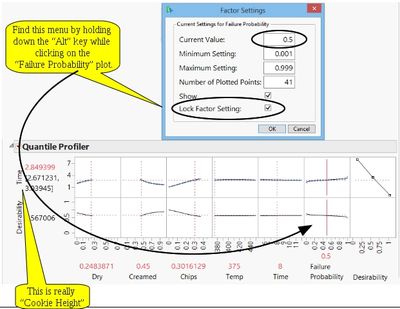
The Optimizer in the Parametric Survival platform treats “Failure Probability” as a factor. This is unnecessary for our analysis, so what should we set it at?
Usually in Response Surface Methodology, we are predicting the mean value. Since we are expecting the logNormal distribution to approximate the Normal distribution, the median should be pretty close to the mean. If we set the “Failure Probability” to 0.5 we should get what we need. Figure 6
Figure 5 – The Parametric Survival Platform |
shows how to “lock” the “Failure Probability” at the median.
Also note that the response will always be labeled “Time.” Of course, you know it's really '”Cookie Height.”
You can add the “Desirability Functions” and set the Desirabilities as usual. You also find the “Sweet Spot” using “Maximize Desirability” as usual.
If you want to make contour plots, you will need to save the prediction formula and use the “Contour Profiler” under “Graph.”
Figure 6 – The Quantile Profiler |
Results
So what did we find?
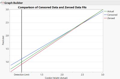
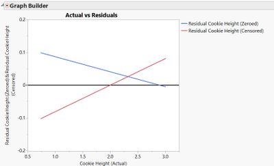
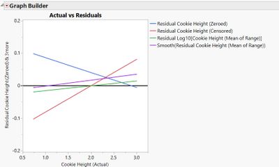
First, we dug up a really good ruler so we could know the actual cookie thickness (this was pretty hard and took a long time ). Then we were able to make an Actual vs. Predicted plot (see Figure 7). This didn't tell the whole story since it left out the noise. So we also created an Actual vs. Residuals plot (see Figure 8). Looking at the the two of these you can see that the results were similar. The residuals were of similar size with a different bias.
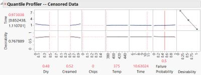
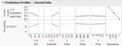
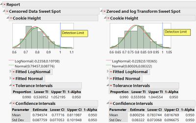
Next we predicted Sweet Spots with both models. Both models predicted essentially the same Sweet Spot, differing only slightly in the predicted baking time (see Figures 9 and 10). We baked 50 cookies for each Sweet Spot and compared the results (see Figure 11).
Figure 7 – Actual vs Predicted Curves |
Figure 8 – Actual vs Residuals Curves |
Figure 9 – The Sweet Spot for the Censored Data Analysis |
Figure 10 – The Sweet Spot for the Zeroed Data Analysis |
The two Sweet Spots yielded the same cookie thickness. We found essentially the same Sweet Spot with both models, so the analysis technique didn't matter for finding a Sweet Spot.
Take a closer look at Figures 9, 10, and 11. Although they predicted the same Sweet Spot, the actual prediction of the censored model was more accurate. Even the confidence limits for the censored model prediction were closer to reality. So if you need accurate predictions, the censored model is better.
Figure 11 – Sweet Spot Comparison |
We really had 2 problems
- We had censored data.
- We needed to model the noise with a distribution that did not predict negative Cookie Heights.
The model with the zeroed data did not address either of these problems. The model accounting for the censored data took both of these problems into account. A natural question is, “Would addressing only one of these problems produce results as good as the censored model?”
While we have no easy way to test problem 1 (we have no way in JMP to look at censored data with a Normal distribution), we can look at problem 2. We can't easily use the Generalized Linear Models platform since it can't be used with mixtures. However, we can make a log transformation of our data and analyze with Standard Least Squares. This has the effect of treating the data as if they were logNormally distributed.
One problem with this approach is that zeroing the data won't work. Instead, we replaced the zeroes with the average of the censored range (0.5). Of course we were still lying to JMP! We also analyzed this data without the log transformation for comparison.
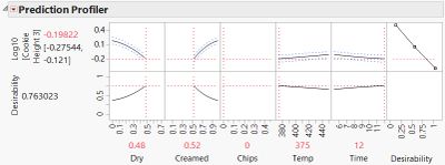
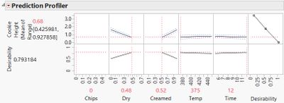
The results for this analysis are in Figures 12 and 13. Notice that the Sweet Spots are identical to the Standard Least Squares fit for Normally distributed data using zeroes. However, the predictions of 0.63 with 95% Confidence limits of 0.53 and 0.76 for the log transformation and 0.68 with 95% Confidence limits of 0.42 and 0.93 for the mean of censored range, are much better than the prediction for the zeroed data analysis. A comparison of all four models is in Figure 14.
Figure 12 – The Sweet Spot for the log Transformation Analysis |
Figure 13 – The Sweet Spot for the Mean of Range Analysis |
Figure 14 – Actual vs Residuals Plots for All Three Models |
You can see that both the censored data model and the log transformed model predicted pretty well – the censored model predicted a little high, the log transformed model predicted a little low. It looks like using the logNormal distribution was not necessary.
Summary
- Assigning “zero” to responses below the detection limit predicted poorly, but yielded a viable Sweet Spot.
- Assigning the mean of the censored range to responses below the detection limit predicted well and yielded a viable Sweet Spot. This is unlikely to work in general – it seems we got lucky this time.
- A log Transformation of the data set in (2) yielded similar results to (2) with a similar caveat.
- Using JMP's Parametric Survival platform with censored data and a logNormal distribution to model the noise predicted well and yielded a viable Sweet Spot for the median. This is likely to work the best in general.
Conclusion
In our work we encountered two problems:
- Censored data
- We needed to model the noise in a way that avoids negative values (at least at the low end).
With our data we were able to solve these problems two ways:
- Analyze with censored data and a logNormal distribution using the Parametric Survival Platform.
- Analyze the log transformation of the data with the censored values replaced by the mean of the range using Standard Least Squares.
As it turned out, the Normal distribution worked fine here – no negative cookie heights predicted.
Both of these methods predicted better than simply zeroing the data below the detection limit. Both methods found essentially the same Sweet Spot.
So what did we really learn?
- Assigning zeroes for unknown values worked well enough. This was probably due to good luck. We would not expect this to work for all data sets.
- Assigning the mean of the censored range worked better, but this was also likely just good luck. We would not expect this to be a good strategy in general.
- JMP's Parametric Survival platform let us analyze the data as censored, although in this case it did not yield better results than the mean of the censored range. In spite of this, this is likely to be the best strategy in the future. While (1) and (2) are simply guesses, the Maximum Likelihood Estimation behind the Parametric Survival Platform is well-established.
- Both the Normal and logNormal distributions worked well for us.
And now we've shared our adventure (and our learning) with you. Now it's time for cookies!
Looking for More?
Here are some interesting references for further information:
Russell B. Millar, Maximum Likelihood Estimation and Inference: With Examples in R, SAS and ADMB, J. Wiley and Sons, 2011, ISBN 978-0470094822.
http://ussynthetic.com/ (for information about US Synthetic)
http://www.ObjectiveExperiments.com (for information about training and workshops)
http://www.jmp.com/ (for information about JMP software)
http://en.wikipedia.org/wiki/Censoring_(statistics) (for a nice explanation of censoring)
http://mathworld.wolfram.com/MaximumLikelihood.html (for a brief explanation of Maximum Likelihood Estimation)
http://en.wikipedia.org/wiki/Chocolate_chip_cookie (for a history of the chocolate chip cookie)
About the Authors
Julie Kidd is a Materials Engineer at US Synthetic. Her specialties are ceramic and composite systems, and materials characterization, including forensic metallurgy and failure analysis.
Heather Schaefer is a Materials Engineer at US Synthetic. Her specialties are cast and pressed energetic materials with an emphasis on infrared decoy flare development.
Together they are currently developing improved synthetic diamonds for the oil and gas industry.
Bill Kappele is President of Objective Experiments. He is responsible for course delivery and development. Julie and Heather learned Design of Experiments from Bill.
Discovery Summit 2014 Resources
Discovery Summit 2014 is over, but it's not too late to participate in the conversation!
Below, you'll find papers, posters and selected video clips from Discovery Summit 2014.
- © 2024 JMP Statistical Discovery LLC. All Rights Reserved.
- Terms of Use
- Privacy Statement
- About JMP
- JMP Software
- JMP User Community
- Contact
